Habitat Modeling - Part 3: Statistical Modeling using MaxEnt
Contents
- Overview - Modeling with MaxEnt
- Step 3.1. Downloading the MaxEnt software
- Step 3.2. Data preparation
- Step 3.3. Running Maxent
- Step 3.4 Model interpretation
- Step 3.5. Mapping the results in ArcGIS Pro
- What’s next
Recordings
- Proj 3.3.1 - Introduction to MaxEnt (3:43)
- Proj 3.3.2 - Maxent Data Prep (10:46)
- Proj 3.3.3 - Running MaxEnt (4:28)
- Proj 3.3.4a - Maxent Predictions (7:34)
- Proj 3.3.4b - Maxent Response Curves (7:30)
- Proj 3.3.4c - Variable Importance (5:06)
- Proj 3.3.4d - Maxent to ArcPro (11:44)
Overview - Modeling with MaxEnt
To complement our rule-based habitat model, we’ll use a statistical approach as well. There are a wide variety of statistical approaches available, GLM, GAM, and CART to name a few. In the interest of time (and also given that this is a GIS course, not a course on statistics), we are going to focus on one of the more popular and robust statistical analysis approaches: MaxEnt.
MaxEnt, released in 2004, uses a maximum entropy approach to determine whether a location is likely to be habitat and what is not. Since its release, MaxEnt has become one of the more popular and widely used species distribution modeling software – and for good reason. MaxEnt is robust and easy to use, it provides insightful output, and it often outperforms other modeling approaches, particularly when observation data is scarce (Elith et. al., 2006).
MaxEnt uses a complex suite of statistical analyses, combining the strengths of neural networks, GAMs, GLMs, envelope models, machine learning – pretty much the kitchen sink of species distribution modeling – into a single “black box”. It’s beyond the scope of this exercise to delve into the mechanics of this black box. For that, I encourage you to familiarize yourself with the MaxEnt “brief” tutorial (40 pages is not exactly brief…) and Elith, et. al. (2011); these are the two most explanatory sources on the MaxEnt approach. Dean Urban’s notes on MaxEnt are also posted on Canvas.
In this exercise, we’ll have a chance to explore some of the nuances of the MaxEnt approach, but mostly we’ll be looking at how ArcGIS and MaxEnt work together to provide a useful means for generating species distribution maps – and understanding more about the ecology of our species.
Step 3.1. Downloading the MaxEnt software
Prior to running this exercise you need to download the MaxEnt executables. The MaxEnt folder contained in the Exercise3_data.zip contains these. Alternatively, you can download them for free from the MaxEnt web site. The contents of the MaxEnt folder are as follows:
- Maxent.jar The MaxEnt executable file. (MaxEnt is written in Java.)
- Maxent.bat A batch file use to run MaxEnt with specific memory settings
- readme.txt A readme file with details on the version of MaxEnt used here
Step 3.2. Data preparation
As it is an inductive model, MaxEnt requires two sets of data: species occurrence points and the environmental layers used to discriminate habitat from non-habitat. MaxEnt is touted to be a “presence-only” platform, and as such we do not need to provide any absence (or even pseudo-absence) data – another advantage of the MaxEnt approach. Here, we discuss the format that MaxEnt requires these inputs to take and how to generate them from the data we already have in our ArcGIS workspace.
3.2.1. Creating the species location file
The first step in running MaxEnt is to generate a list of presence localities, or “samples”. In its simplest form, this is simply a CSV file with three columns: a species column listing the name of the species that a given sample represents, and columns for the X and Y coordinates. The order of the columns is important: the species column must always come first, followed by the X coordinate and then the Y coordinate. An example is shown below (this example is from the sample data that comes with MaxEnt).
species,longitude,latitude
bradypus_variegatus,-65.4,-10.3833
bradypus_variegatus,-65.3833,-10.3833
bradypus_variegatus,-65.1333,-16.8
bradypus_variegatus,-63.6667,-17.45
bradypus_variegatus,-63.85,-17.4
You can have as many species as you want in your samples file, as long as they are labeled uniquely in the first column. MaxEnt will allow you to select individual species (or all species) when you run an analysis. So, our first task is to create this CSV file for our salamander.
You can generate this easily from the PigmySalamander_South.shp shapefile by exporting its feature attribute table to a CSV text file using the Export Table tool, being sure to give the filename a .csv extension. You can then edit the resulting text file in Excel to (1) add a column for species name and (2) delete/re-order the columns so that the X (“easting”) and Y (“northing”) fields follow the species name.
Note: if your attribute table did not contain the X and Y coordinates, use the Add XY Coordinate tool…
3.2.2. Creating the ASCII format environmental layers
Our next objective is to convert all the environmental rasters that we created in the first lab into a format that MaxEnt can read, which is ASCII format. The one major catch in creating these ASCII rasters is that for them to be read into MaxEnt, they must have the exact same cell size, alignment, and extent. Furthermore, since MaxEnt will use these ASCII files to extract values at our sample locations, these rasters must have the same coordinate system/projection that our sample coordinates use. Fortunately, as we took extra care in setting the proper environment variables when we created our environmental layers, this should be a relatively straightforward task.
You could create a new geoprocessing model and add 16 instances of the Raster to ASCII format, but there’s an easier way with a simple advanced modeling trick. To do this:
-
Create a new geoprocessing model and add one instance of the Raster to ASCII tool.
-
Then from the Insert panel of the Model Builder toolbar, add the Iterate Raster iterator to your model. This will add a means by which you can iterate through all rasters in a given workspace.
-
Open the iterate Rasters object in the model and specify your
EnvVars.gdbgeodatabase containing all your environmental variables. Leave the remaining options blank. The output to this object now appears to be the first raster in your folder. Connect this to your Raster to ASCII tool. -
Open up the Raster to ASCII tool and set the output to go to a new, empty folder. (e.g. create a new folder called
ASCIIin your Data folder and select the output to go in there. For the file name, enter %name%.asc. The result should resemble this: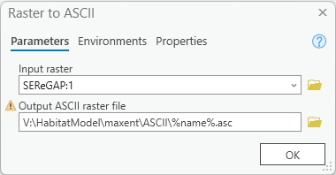
What this does is iterate through each raster found in the folder you specified, convert it to raster and, with each iteration, the “Name” variable contains the current raster the model is processing (e.g. “Elevation” for the first run, then “USA_GAP_LandCover”, etc.), and the output is given this name.
Run the model and you should have 17 ASCII files in your ASCII folder when complete.
Note: If you have to re-run this model, or any model with an iterator element in it, be sure to validate the model first as it will reset the iterator.
Step 3.3. Running MaxEnt
MaxEnt can be run by double-clicking the maxent.jar file in your MaxEnt folder. Another way to start MaxEnt is to double click on the maxent.bat file. Why the difference? Well, the maxen.bat file just calls the maxent.jar file, but the maxent.bat file can be edited in a text editor to run MaxEnt with more than the default 512 Mb of RAM allocated to it. The machines in the ICL and ACL have 8 GB of RAM, and we can run MaxEnt a lot faster if we allow it to consume more memory when its run. To do this we edit the maxent.bat file, changing the 512 Mb to 2048 Mb so it runs with 2 Gb of memory instead of ½ Gb.
3.3.1. Running MaxEnt with more memory
-
Edit the maxent.bat file in a text editor.
-
Change “512m” to “2048m“
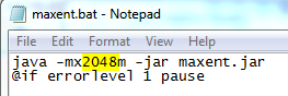
-
Save and close the maxent.bat file.
-
Double-click the maxent.bat file to run MaxEnt.
MaxEnt should now appear and we’re ready to set up our analysis
3.3.2. MaxEnt inputs and run-time settings
With MaxEnt up and awaiting our command, we now have to specify the samples file, the folder containing our ASCII format environment variables, and output folder, and a few run-time settings. These steps lead us through this process:
-
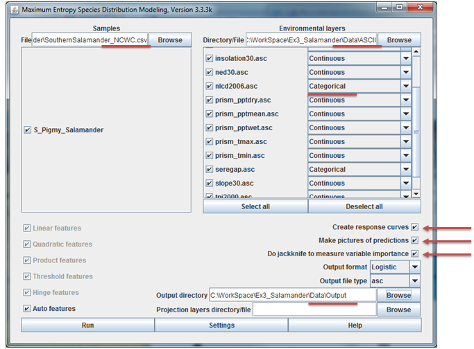
Specify the samples dataset by browsing to the
csvfile we created in the data preparation section above. You should see the salamander species appear with a check box next to it. Keep all selected as we’ll run all species simultaneously. -
Specify the folder containing all your ASCII formatted environment layers. When entered, a list of all the rasters in the folder will appear, each with a check box next to them. Notice that you can add categorical data in MaxEnt. Make sure that you set the two land cover datasets to be categorical data.
-
Specify an output folder. In specifying this folder, you can create a new folder. Create a new folder in your MaxEnt folder and set all model output to go here.
-
Set the following run-time settings:
a. Check the box to create response curves
b. Check the box to make pictures of predictions
c. Check the box to do jackknife to measure variable importance
d. Keep output format as Logistic
e. Keep output file type as asc
The MaxEnt application should resemble the figure below. When all is set, hit Run. You may see a few errors for field names that were not used and perhaps for a few points falling outside of the environmental extent. You can just ignore these. The program should finish in about 5-10 minutes or so.
Step 3.4. Model interpretation
MaxEnt generates a lot of output, all indexed through a web page created in your output folder. Here we’ll run through the highlights of the output. Your report may have slightly different values as each run of MaxEnt extracts a random sample of background points, but they shouldn’t be too different. Open up your S_Pigmy_Salamander.html file in any web browser and follow along…
3.4.1. Viewing the prediction raster
For now, we’re going to skip the first two graphs (“Analysis of omission/commission” and “Sensitivity vs. 1 – Specificity”) and the first table. We’ll come back to those when we discuss model assessment in a future exercise. Instead, scroll down to the map of the study area painted in blues to reds (“Pictures of the model”)
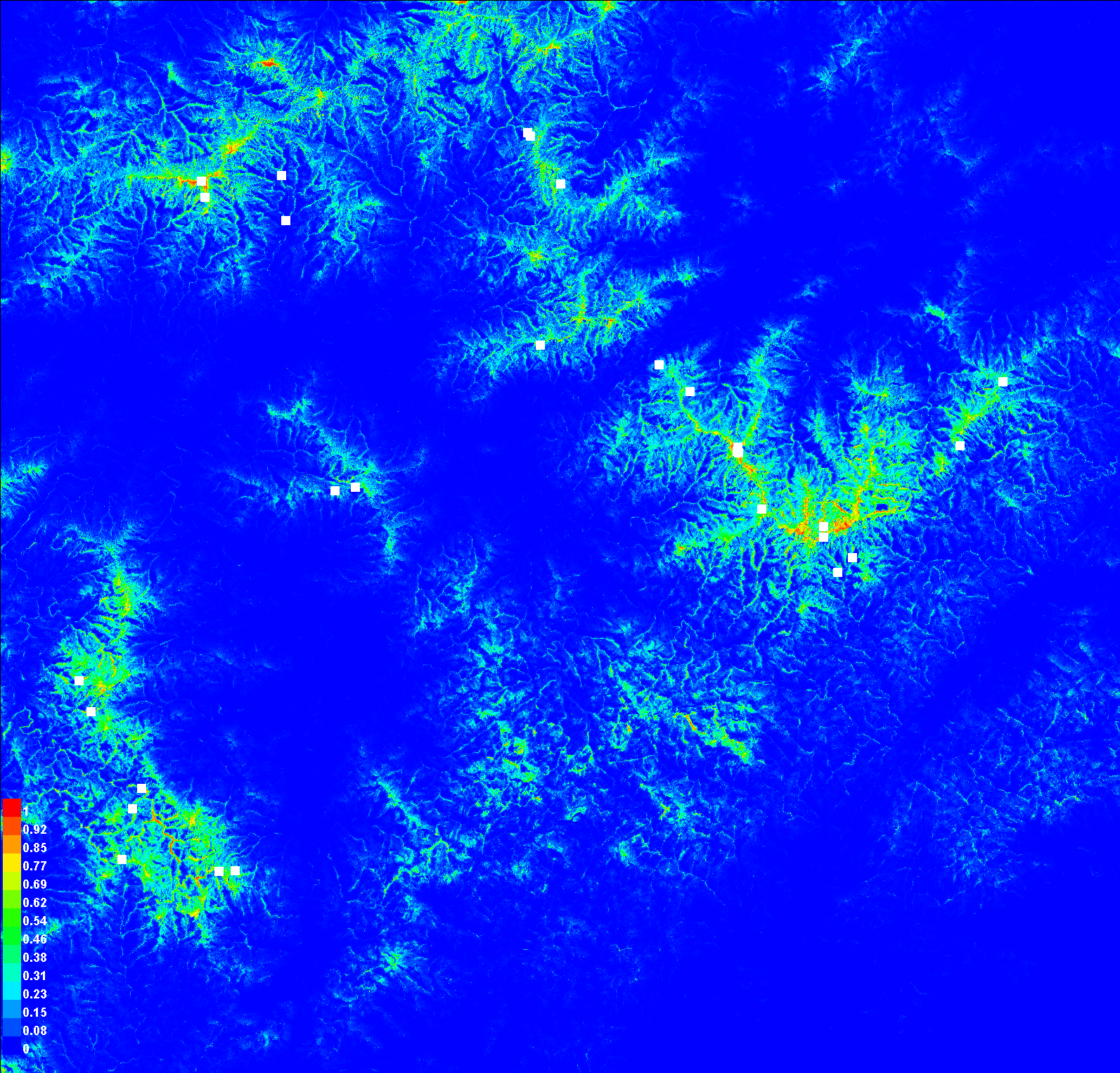
This is our habitat suitability map as predicted by MaxEnt. The values range from 0 to 1. The closer a cell’s value is to 1 (the warmer colors), the more confident we are that the pixel represents suitable habitat. This is not quite a habitat map, as we still need to decide on a cutoff for what we want to be habitat or not, but we’ll get there. First, let’s explore how MaxEnt arrived at this map.
3.4.2. Reading the response curves
Scroll down to the section on Response Curves. The first group shows the marginal response curve for each environmental variable. In these line graphs, the X axis reflects the range of values for the given environment variable and the Y axis reflects the likelihood of habitat at that given range. Flat lines indicate that the variable has no real influence in separating habitat from non-habitat. The shape of the response curve reflects the various methods that MaxEnt uses to model responses (categorical, linear, quadratic, threshold, hinges, and/or interactions). As an example, have a look at the “prism_tmean_min” response curve (below). This flat response curve suggests that mean monthly temperature does not add much marginal predictive power, meaning power beyond what the other variables can provide.
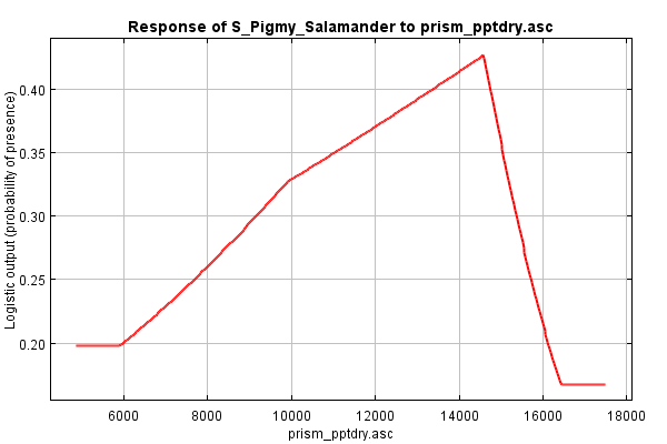
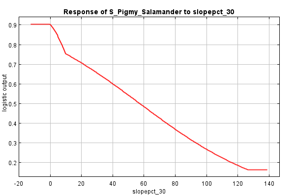
Contrast this with the marginal response curve of slope. This curve suggests that slope interacts with other variables such that habitat preference is highest in areas of low slope and steadily declines as slopes increase, with a subtle bend in the curve at around 10% slopes.
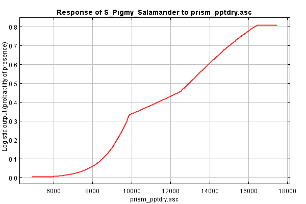
Now, let’s move down to the next set of response curves, the dependence response curves. These curves are generated using only the corresponding variable; all others are ignored. Thus, the responses shown are independent of interactions among variables, showing only the single variable’s contribution to predicting habitat.
First, we revisit mean temperature: it’s no longer flat! Instead, we see that, if we were to only look at temperature, salamanders appear to prefer cooler areas than warm ones, with areas below ~7.6°C being equally favorable and areas above ~14.5°C being equally unfavorable. Why don’t we see this difference in the marginal response curve? Because the response is likely already captured in some other variable. (Elevation??)
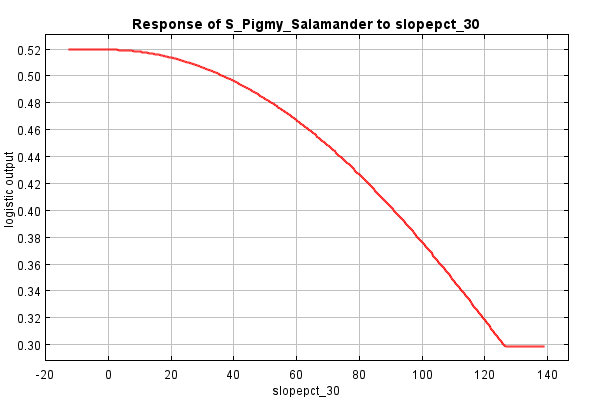
And what about slope? The direction seems to be the same (lower habitat likelihood as percent slope increases), but the shape is a bit different, a bit rounder. The difference between the two curves is a bit smaller, perhaps suggesting that slope’s impact on discerning habitat from non-habitat is independent from interactions other variables.
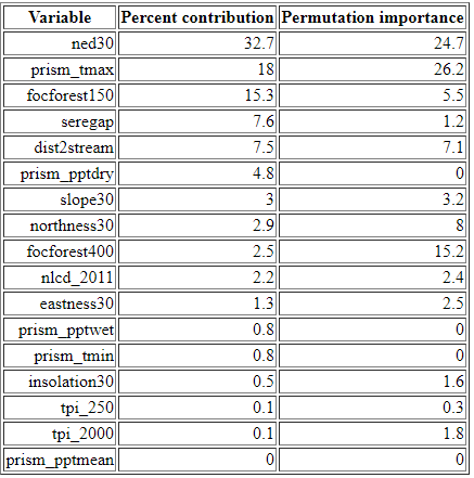
3.4.3. Analysis of variable contributions
In this section of the MaxEnt output file, we can see the relative importance of each environment variable in driving the final habitat suitability surface. The table lists each variable in order of its percent contribution to the model’s gain. Gain is a measure of improvement to the model’s ability to separate habitat from background, i.e., from retaining areas that include the values specified in the occurrence locations but removing all other areas (or “background”). As the MaxEnt tutorial cautions, the percent contribution listed in the table should not be over-interpreted as they reflect just one pathway to an optimal solution (and there may be many). Still, the table does provide at least a rough guide showing which variables appear to be important in determining habitat for a given species.
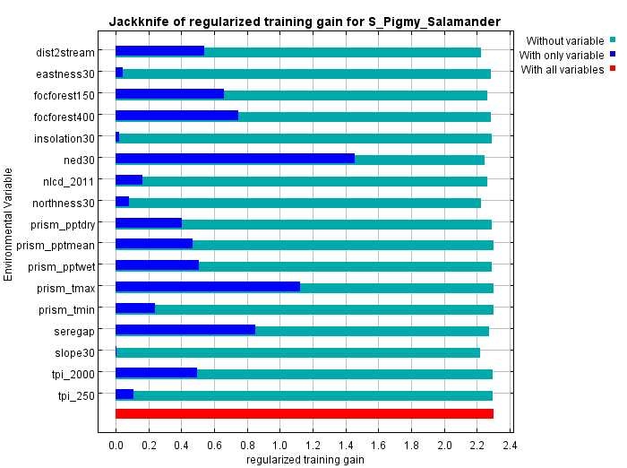
3.4.4. Interpreting the jackknife figure
The jackknifing figure (below) provides a different view of the relative importance of the different variables. In the figure below for our salamander, the short dark blue bar for slopepct_30 indicates that it, by itself, contributes very little gain (or ability to separate habitat from background). Conversely, elevation , which has the longest dark blue bar, contributes the most to gain. We can interpret this as: if we were limited to choosing only one variable to parse habitat from background, we should chose elevation of as it would give us the best single-variable model.
 {
{
The lighter blue bars show the decline in gain if a variable were omitted. It’s a way of spotting whether a variable contributes something unique to the solution. In our example, slope, or perhaps usa_gap_landcover, shows the biggest drop in gain when omitted implying that, when it’s removed, there’s no other environmental variable that captures its contribution to gain. However, the difference is slight suggesting that the impact wouldn’t be too large if the variable were omitted.
Model Interpretation: Overview
The key product from our MaxEnt analysis is the ASCII format raster of representing habitat likelihoods which we will shortly pull into ArcGIS. But the above digest of what variables are important and their response curves are also quite useful in understanding the ecology of each species distribution. Knowing the relative importance of a given environmental variable gives us insight into what factors may be constraining our species’ distribution. And knowing the response curve gives us an idea how: is it a monotonic relationship? Or is there one or more “sweet spots” that the species seem to prefer.
In the case of our salamander analysis, we see that the elevation, maximum monthly temperature, and GAP land cover stand out as providing the most gain when modeled alone and leads to the largest decline in gain when omitted. So it seems that these factor seems to be important to the salamander.
Step 3.5. Mapping the results in ArcGIS Pro
The last remaining step is to bring MaxEnt’s logistical output, in the form of an ASCII raster, back into ArcGIS, and then apply a threshold to map the habitat ranges for each of our species.
-
Create a new geoprocessing model to process the MaxEnt outputs.
-
Add the Copy Raster tool to convert the Maxent prediction ASCII output to an ArcGIS raster dataset. If you look at the ASCII file in a text editor, you’ll see the NoData value is -9999. The values range from 0 to 1, so we want to preserve decimals in our output, not convert them to integers. The only option in the Pixel type that produces floating point output is “32 bit float”. Save the raster in your project geodatabase.
-
The ASCII files generated do not know what coordinate system they are in, so we need to define that. Add a Define Projection tool at the end of each ASCII to Raster tool to define the outputs to have the coordinate reference system used by our other datasets.
Run the model and view the MaxEnt logistical outputs. Values in these rasters should range from 0 to 1, with the higher values indicating a higher likelihood that the pixel is “habitat”. The next step is to apply a cutoff. The decision where to draw the line between habitat and non-habitat is not arbitrary and depends on the sensitivity and specificity of the model (terms we’ll discuss shortly). We’ll discuss model tuning in a future lecture, but for now I’ll just point you to the value in the MaxEnt results that gives us a good cutoff.
If you scroll to the top of your species’ MaxEnt report, to the table that list Cumulative threshold, you’ll see a series of logistic thresholds for different criteria. The table for our salamander is shown below.
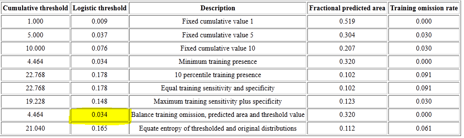
These logistic thresholds (column 2) are the cutoffs to separate habitat from non-habitat, and the one most often used is the second from the last, the “Balance training omission, predicted area and threshold value”. Your values may be different based on the set of random background points selected and the model surface generated by MaxEnt
The remaining steps are to use these thresholds in Test tool to assign cells that are ranges for our given species as 1 and all other values as 0. The result will be our species habitat map derived from MaxEnt.
What’s next
In the continuation of this lab, we will review the techniques presented here and focus in on the assessment and interpretation of our distribution models. Ultimately, you will submit a brief report assessing your habitat model of the pygmy salamander.
References
Austin, M.P. (2002), Spatial prediction of species distribution: an interface between ecological theory and statistical modeling. Ecological Modelling, 157: 101-118. http://www.sciencedirect.com/science/article/pii/S0304380002002053
Elith, J., et al. (2006), Novel methods improve prediction of species’ distributions from occurrence data. Ecography, 29: 129–151. (http://onlinelibrary.wiley.com/doi/10.1111/j.2006.0906-7590.04596.x/abstract)
Elith, J, et al. (2010), A statistical explanation of MaxEnt for ecologists. Diversity and Distributions, 17: 43 - 55. http://onlinelibrary.wiley.com/doi/10.1111/j.1472-4642.2010.00725.x/pdf
Phillips, S. (2006), A brief tutorial on Maxent. AT & T Research. (http://www.cs.princeton.edu/~schapire/maxent/tutorial/tutorial.doc)