Habitat Modeling Project - Part 2: Rule-Based Modeling
Contents
Recordings
- Proj 3.2.1 - Rule Based Analysis -Intro (4:01)
- Proj 3.2.2 - Model Builder Approach (11:12)
- Proj 3.2.3 - Raster Calculator Approach (5:00)
- Proj 3.2.4 - Jupyter Notebook Approach (5:34)
Overview - Rule-based modeling
Rule-based habitat models, also referred to as generative or envelope models, are the oldest and simplest habitat models. They consist of defining the limits of different environmental conditions in which one would expect to find a species - the so-called “Hutchinsonian hypervolume”. The trickiest part of these rule based models is defining the limits. This is most often done using expert knowledge about the species, but could also be done using observation data to chart - in parameter space - the ranges in which the species has been observed. Envelopes or Mahalanobis distance metrics can be applied to these values to confine the hypervolume, but once the boundaries are specified, the spatial component is relatively easy.
In our exercise, we will rely on “expert knowledge” about the pigmy salamander. We’ll use this knowledge to set the rules and then use some raster algebra to apply those rules to come up with habitat map for our species.
Step 2.1. Setting the rules
From our background research as well as meetings with pigmy salamander experts, we’ve deduced the following constraints on our salamander.
-
Salamanders are found above 762 m in elevation and below 2012 m.
-
Salamanders prefer areas that are within 400 m of the following GAP cover classes:
-
Class #63 - Central and Southern Appalachian Northern Hardwood Forest
-
Class #84 - Southern and Central Appalachian Oak Forest
-
Class #96 - Central and Southern Appalachian Spruce-Fir Forest
-
-
Salamanders require places where the monthly average temperature never exceeds 22° C.
-
Salamanders occur in places where the driest month averages at least 96mm of precipitation.
Step 2.2. Applying the rules
With out underlying goal to learn more about GIS, we will explore a few ways to apply these rules to generate our rule-based habitat map.
2.2.1 Step by step approach in the the Model Builder
First, we’ll build a geoprocessing tool that creates binary rasters of each rule and then combines them such that only pixels meeting all criteria get assigned a “true” value, i.e., a value of “1” with all other pixels assigned a zero.
- Create a new geoprocessing model:
5. Rule-based analysis - Add 4 instances of the
Testmodel, recalling that this model creates a binary raster from an input raster and a “where clause”. - Add the following rasters from your
EnvVars.gdbgeodatabase to the model:Elevation,FocForest400,PRISM_TMEAN_max, andPRISM_PPT_min. - Use these
Testtools to apply the 4 constraints listed above, with the products going to the scratch (ormemory) geodatabases.- Note carefully which comparative operator to use for each constraint, e.g.
<or<=?
- Note carefully which comparative operator to use for each constraint, e.g.
- Use the
Cell Statisticstool to combine these to produce an output where only pixels set as 1 in all of the 4 inputs is assigned a 1 as the output. This output should go to your default project geodatabase. Call it “RuleBasedHabitat_1”,
2.2.2 Using the Raster Calculator
Next, we’ll explore how all this can be done in a single tool: the Raster Calculator
-
Add the
Raster Calculatortool to your5. Rule-based analysismodel. -
Enter the following calculation, setting the output to go to your project geodatabase as “
RuleBasedHabitat_2”( "%Elevation%" > 762) & ("%Elevation%" < 2012) & ( "%FocForest_400%" > 0.5) & ( "%PRISM_TMEAN_max%" <= 2200) & ( "%PRISM_PPT_min%" >= 9600)
Separate “Test” tools or a single “Raster Calculator”?
Both methods above should produce the exact same result. Do you prefer the efficiency of the Raster Calculator, or are you put off by how difficult it can be to type the expression? What other advantages and disadvantages do each approach provide.
2.2.3 Using a Jupyter Notebook
Finally, we’ll examine raster calculations using Python, written in a Jupyter Notebook. Again, we won’t be going into detail on Python scripting here. Rather I just want you to see this alternative in action as a potential 3rd option.
- If you don’t already have a Scripts folder in your project workspace, create one.
- Place the
RuleBasedAnalysis.ipynbfile located here into the Scripts folder. This.ipynbfile is a Jupyter notebook file. - From the ArcGIS Pro Catalog Pane, find and open the “RuleBasedAnalysis” notebook.
- Run each code cell sequentially by clicking the ► button in the notebook toolbar.
The result will be added to your map and saved to the Scratch geodatabase (unless the script is unable to find the EnvVars.gdb or Scratch.gdb).
What do you think of the notebook based approach? Advantages? Disadvantages?
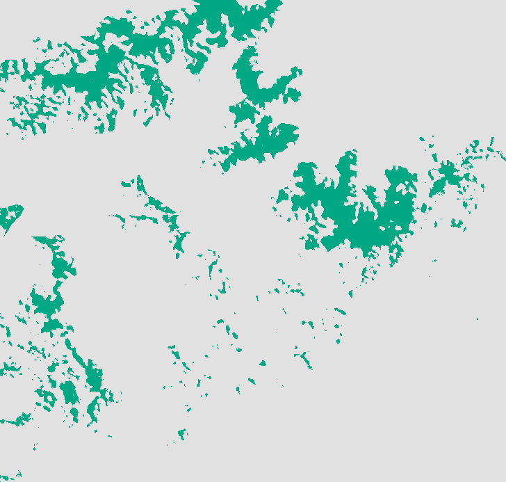
The output is your rule-based prediction. It is the spatial representation of the conditions that the experts believed to be real constraints on the salamander’s habitat. Your result should resemble this:
Summary
Not much to rule based modeling. We simply isolate the pixels that match the rules. Its elegance is in its simplicity, but the result is a pretty stark binary map. We have no indication of how close a pixel was to being ruled out or ruled in, no way of tuning our result to be more sensitive to including possibly misclassified habitat or excluding possibly misclassified non-habitat.
And this is why we continue with a second way of modeling habitat, so called discriminant analysis where we look beyond applying rules in a binary fashion, but rather look at the likelihood that a pixel meets a given criteria as well as how important that particular criteria is in determining whether the pixel is actually habitat or not.