Lab X: Demographics & Dasymetric Mapping
Overview
Here we will download and examine census data to explore any relationships between demographics and CAFO locations. We'll focus on Duplin Co. We'll examine the finest resolution publicly available census data, i.e. blocks, and the various attributes associated with each. We will also examine basic techniques of dasymetric mapping, a technique used to extrapolate aggregated data, such as population within a block group, to much finer scales, e.g. a pixel.
Census data structure
Census data consist of two parts: geographic entities and attribute data. They are linked using FIPS codes. (You may also see these called GEOID in some more recent datasets.)
The geographic entities come in different aggregated sizes: State, County, Tract, Block Group, and Block. These entities are diagrammed here: http://www2.census.gov/geo/pdfs/reference/geodiagram.pdf. Each entity is labeled by its Federal Information Processing Standard, or FIPS code. FIPS codes are hierarchical in that larger units have fewer digits (e.g., NC has the FIPS code '37'), and smaller units build off these values (e.g., Durham Co. is FIPS Code '37063'). Thus each geographic entity has a unique FIPS code that reveals the larger entity into which it belongs. These unique FIPS code also enable Census attribute data to be attached to these geographic features.
The Census (and other entities) provide countless raw, aggregated, and statistically interpreted tables via the American Fact Finder web site https://factfinder.census.gov). These include data from the decennial census of all Americans, but also the American Community Survey, which collects more detailed information on a sample of Americans. These data have a finer temporal resolution with 1, 3, and 5 year estimates.
Obtaining Census data
We can find census data from ESRI’s Living Atlas:
-
From the catalog pane in ArcGIS Pro, select Portal then the Living Atlas icon.
-
Search for USA Census Tracts and select the USA Census Tract Areas from the results and add this item to your map. This dataset has an attribute for the population estimate in 2014.
-
Create a layer from this dataset that is the subset of the counties on which you want to perform dasymetric analysis.
- NC FIPS = 37
- Durham FIPS = 063
Dasymetric Mapping
Dasymetric mapping is a "technique in which attribute data that is organized by a large or arbitrary area unit is more accurately distributed within that unit by the overlay of geographic boundaries that exclude, restrict, or confine the attribute in question." We will use dasymetric mapping to estimate where the X number of people occupying a given census spatial unit (tract/block group/block) are likely distributed within the unit based on the distribution of land cover within that unit.
The process requires three pieces of data:
-
The polygon features of the generalized data, often called the enumeration unit. We'll use the census blocks with associated population data we obtained above.
-
A finer grained dataset from which we can estimate the likely relative density of people. This is often, though not always, a land cover dataset. We'll be using the 2011 NLCD.
-
A table listing the likely relative density of people in each class of the above finer grained dataset. This is perhaps the most subjective of the three inputs. Mennis (2003) describes a sampling scheme to get at more precise values, but we will use general estimates for this exercise.
From these three pieces, we will use the following formula to compute the population at each pixel within a county (taken from Holloway et al., 1996):
\(P = ((R_A *(P_A~/ P_A))*N/E)/A_T\) Where:
-
P is the population of a cell,
-
R_A is the relative density of a cell with land-cover type A.
-
P_A is the proportion of cells of land-cover type A in the enumeration unit,
-
N is the actual population of enumeration unit (i.e., census block)
-
E is the expected population of enumeration unit calculated using the relative densities. E equals the sum of the products of relative density and the proportion of each land-cover type in each enumeration unit.
-
$A_T$ is the total number of cells in the enumeration unit.
P_A / P_A, which cancels each other out, is to calculate the unit area in the grid-based dasymetric mapping method. The output population is estimated for each cell, not for each mapping unit (in the vector approach). The cell size of the land-cover layer is 30 by 30 m. You need to divide the area of the enumeration units by 30 x 30 to get the value of A~T~. The values of R~A~ for different land-cover types are provided as follows.
| NLCD Class | DESCRIPTION | Relative Density ($R_A$) |
|---|---|---|
| 11 | Open Water | 0 |
| 21 | Developed, Open Space | 5 |
| 22 | Developed, Low Intensity | 50 |
| 23 | Developed, Medium Intensity | 10 |
| 24 | Developed, High Intensity | 10 |
| 31 | Barren Land | 1 |
| 41 | Deciduous Forest | 5 |
| 42 | Evergreen Forest | 5 |
| 43 | Mixed Forest | 5 |
| 52 | Shrub/Scrub | 1 |
| 71 | Herbaceuous | 1 |
| 81 | Hay/Pasture | 5 |
| 82 | Cultivated Crops | 2 |
| 90 | Woody Wetlands | 0 |
| 95 | Emergent Herbaceuous Wetlands | 0 |
Analysis procedure
The general procedure for implementing this process is provided here:
-
Convert the NLCD raster in to a raster of relative densities using the table provided.
-
First, subset the NLCD to the area of the county using Extract by Mask.
-
Then, reclassify the NLCD values into relative densities using the table provided. For this you can use the Reclass By Table tool and the RelativeDensity.csv file provided in the workspace.
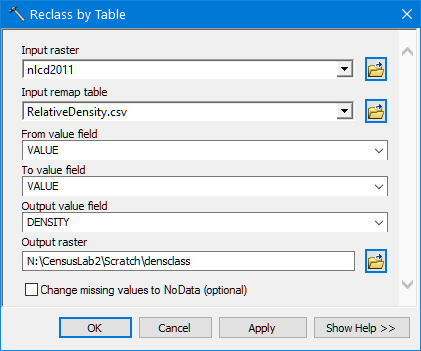
-
The output should be a raster of six values - 0, 1, 2, 5, 10, and 50 – reflecting population density relative to each other. For example, a pixel with a value of 10 would, hypothetically, be twice as dense as a pixel with a value of 5.
-
-
Generate a table listing the number of pixels within each relative density class falling within each census block.
-
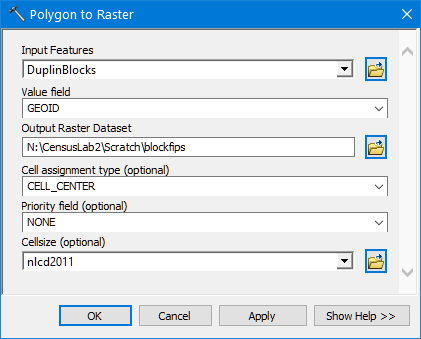
First we must convert our census block polygon features to rasters, using the GEOID (i.e. the 15 digit FIPS code) as the value field. We do this with the Polygon to Raster tool.
-
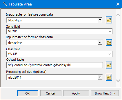
With this we use the Tabulate Area tool to cross tabulate the area (in m2) of each relative density class falling within each block feature. It's best to save this output as a geodatabase table to preserve long field names. So you may wish to create a geodatabase in your scratch folder to hold this table.
-
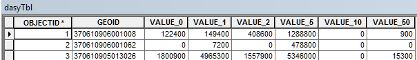
The result should list each block as a row and a column for each of the relative area class.
-
-
Convert these area values into proportions. To do this we need to add Total field and proportion fields for each of the 6 density classes and then compute the proportion of each class by dividing the area by the total area. This is a tedious process that can be done manually or within a geoprocessing model, I've constructed a model to do this for you (as well as a Python script where it's much easier). However, the steps are provided below.
-
Add a new double precision field called "TOTAL".
-
Compute values of the TOTAL field as the sum of the Value fields:
[VALUE_0]+ [VALUE_1]+ [VALUE_2]+ [VALUE_5]+ [VALUE_10]+ [VALUE_50] -
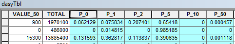
Add 6 new double precision fields for each of the relative density classes: P0, P1, P2, P5, P10, and P50.
-
Compute these fields as the respective VALUE field divided by the TOTAL field: e.g,
[VALUE_0] \ [Total] -
The resulting columns should appear like this:
-
-
Now we can compute "E", the expected population per block, using the population densities per cell calculated in the previous step. The value of E is decided by the proportions of land-cover types in each census block, not by the actual population of the block reported in the census. The value of 'E' is important as it lets us rescale our relative densities into actual population estimates.
Here's an example of how that works: Say a census block has a computed expected value of 'E' = 4, but the actual population reported by the census for the block is 32, or 8x the expected value. If that's the case, we can multiply all our relative density values by 8 to get actual densities.
The 'E' field values are computed in the script tool I provide, but if you want to compute by hand, here’s how.-
Add another double precision field to your table. Name it 'E'.
-
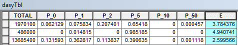
Compute it as the sum of each proportion column multiplied by its density value:
[P1] + 2 * [P2] + 5 * [P5] + 10 * [P10] + 50 * [P50] -
This should appear as follows:
-
-
Again, the significance of the table created above is that it includes, for each census block, the conversion factor, namely the ration of E to actual population, to rescale the relative density values into actual density values, from which we can estimate population at the pixel level. So our next step is to do just that: convert our relative densities into actual densities.
Recalling the original equation: P = (R~A~*N/E)/A~T~, we compute P at the pixel level by applying the raster calculator on rasters for each component in the equation. P = ((R~A~*(P~A~/ P~A~))*N/E)/A~T~
-
We get R~A~ from the reclassified NLCD raster compute above
-
N is obtained by converting the block feature class to a raster on the population attribute.
-
E is converted to a raster by joining the dasyTbl to the blocks and converting that to a raster based on the E attribute.
-
And A~T~ is the Total column in the dasyTbl which we again join to the block attribute table and convert to raster.
And here are the step-by-step instructions:
-
First create a copy of your block feature class. We're going to write new attributes to its table, so it's best to do this on a copy of the original data… Use Copy Features for this process.
-
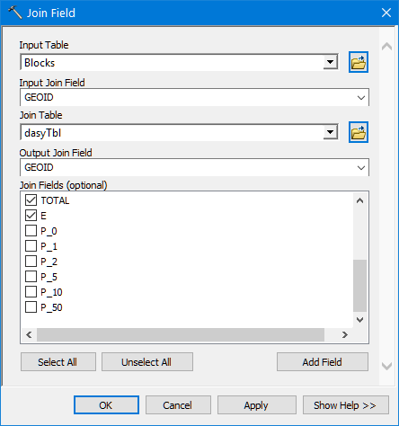
Next use the Join Field tool to append the TOTAL and E fields from the dasyTbl table to the copied Block features.
-
Use three instances of the Polygon to Raster tool to convert the block population (D001), TOTAL, and E fields to rasters. I'll refer to the outputs as "BlockPop", "Block_Tot", and "Block_E", respectively. Be sure to set the output cell size to the same as the Relative Densities raster (30).
-
Compute population in the Raster Calculator tool by multiplying the Relative Densities by the Block Population output and divide by the product of 'E' * 'TOTAL':
("%Relative densities%" * "%BlockPop%") / ("%BlocksE%" * "%Block_Total%") -
This result gives the # people per m2, so to increase to pixels we multiply by the pixel area to represent people per 30 x 30 pixel:
("%Relative densities%" * "%BlockPop%") / ("%BlocksE%" * "%Block_Total%") *** 900**
And the result is population at a 30 x 30 m cell size created by dishing out the block level population across pixels within the block – assigning more population to pixels with a higher expected relative density!
Display your result as stretch values, setting pixels with zero population as a distinct color. How does it look? Pull in the CAFO data: how many folks are expected to reside near hog farms?