Lab 5: Conservation Planning - Calculating Biodiversity


Preparation
Introduction
1. Upscaling Habitat Patch Metrics to Landscape Planning Units
2. Biodiversity Calculations
2A. Estimating richness from GAP cover data
2B. Data visualization
2C. Estimating evenness from GAP cover data
3. Creating Biophysical Zip-Codes
3A. Steps to Create Zip Codes for the Mogollon Plateau
Summary
Deliverables
Preparation
Download the BiodiversityLab.zip file expand it in your class drive. View the Readme.txt file for descriptions of the datasets, models, and scripts provided in this workspace. Refer to the end of this document for a list of the deliverables to submit for this exercise.
Introduction
Scaling up: From Habitat Assessment to Conservation Planning
Over the past few weeks, we’ve calculated a number of habitat patch metrics relating to patch size, shape, dispersion, and connectivity. These metrics can be easily assembled into a single database (by attribute joining) that allows us to sort and rank habitat patches according to various conservation priorities.
While these habitat patch attributes will certainly be important in devising a conservation plan for the Mogollon Plateau, constraining our analysis only to where habitat occurs neglects opportunities (and threats) which may occur outside habitat areas. Therefore, in the next few labs we expand our prioritization analysis from the habitat patch to landscape planning units so that our conservation planning includes a more comprehensive evaluation of the landscape.
The Landscape Planning Unit
Like habitat patches, landscape planning units are defined, contiguous areas that we assess for their relative contribution to various conservation objectives. How we divide a landscape into planning units can depend on a variety of factors.
-
Land tenureship or administrative boundaries (e.g. ownership parcels) can be useful as they often align with the factors of acquisition and protection. However, these data can be difficult to obtain and may be inconsistent across the extent of the landscape (e.g. from one county to another).
-
Arbitrary units such as tessellated blocks or hexagons can be generated for any landscape and offer consistent (and objective) landscape units.
-
Geographic features such as roadless areas (areas bounded by roads) or catchments make for objective, ecologically meaningful units, but may not associate well with likelihood of protection (cf. administrative boundaries).
-
Lastly, arbitrary or custom drawn regions such as park boundaries and protected areas allow maximum flexibility in designating areas, but are seldom as objective or systematic as other methods.
Planning unit attributes – An example: EPA’s EnviroAtlas
Once the planning unit, or “PU” scheme has been defined, we can begin assigning attributes to each PU. The number and range of attributes we can assign is limitless and depends on the conservation objective. A good example of this, the EPA’s EnviroAtlas (http://enviroatlas.epa.gov/enviroatlas/atlas.html) which provides a national coverage of 12-digit HUCs (“HUC 12s”) planning units with several dozen attributes. As we will see later, these attributes, like habitat patch attributes, can be combined using various methods to arrive a single ranking of HUCs so that we may arrive at an objective and comprehensive conservation plan.
Our Lab Exercise – Calculating Habitat and Biodiversity for HUC 12 Planning Units
Meanwhile, we return to our Mogollon Plateau landscape and use HUC12s from the National Watershed Boundary Database (http://nhd.usgs.gov/wbd.html) as our planning units. While these range in size from 30 to 180 km2 and are clipped at the boundary of our landscape, they serve a useful template for devising a conservation plan.
We begin our exercise with techniques used to upscale our habitat patch attributes to into value at the planning unit scale, and then continue with some procedures for calculating biodiversity metrics. From there, in subsequent labs, we will look at mapping threats and habitat stressors and assign additional attributes to these planning units. And ultimately we will examine methods used for combining these metrics to meet conservation objectives and arrive at a conservation plan for the landscape.
1. Upscaling Habitat Patch Metrics to Landscape Planning Units
NOTE: In the interest of time, Part 1 of this assignment – upscaling habitat patch metrics – has been completed for you. This doesn’t mean you can just skip to Part 2 but rather you should walk through the procedure, tools, and results yourself so that you have a solid understanding what is happening. If you have any questions, don’t hesitate to discuss with the instructor, TAs, or even your classmates.
From previous labs, we have a list of patch attributes and we need to carry these over to our HUC 12 landscape planning units. For the most part, this is as straightforward as identifying whether we should take a sum or mean of the values, but there is one important catch: several habitat patches span across two or more planning units. That being the case, if we include one HUC 12 in the conservation plan but not another, we would only be protecting the portion of the habitat patch in the one.
The solution to this issue is to split the patches across planning units and recalculate habitat patch geometry and connectivity scores. This is not a perfect solution as patch shape index and core-area ratios will change as we artificially fragment our patches across planning units. Ideally, we’d recalculate these metrics under all planning unit selection configurations (e.g. if we select patch 2 and 3, patch “X” fuses and becomes a much more valuable patch), but the calculations involved quickly get out of hand. That said, we will examine software that “solves” this issue. Additionally, our connectivity metrics approximate the benefit of choosing planning units that connect patches.
1A. Updating attributes of patches subset by planning unit
To save time, we’ve provided you with a tool
1. Calculate Patch HUC Metricsin theBiodiversityTools.tbxtoolbox that does the following analysis. You should NOT run this too as it takes a long time (> 3 hours!), but you should understand how it works and what it’s doing…
This tool splits the pronghorn habitat patches across HUC 12 planning units – using the Combine tool – and recalculates both patch geometry and patch connectivity scores. See the Calculate Patch HUC Metrics tool in the Recalculate Patch Metrics toolset. This tool includes sub-tools to [re] calculate both patch geometry and patch connectivity metrics. If executed it for you as it can take a long time to complete (~45 minutes for creating the edge list). The result is the HUCPatches dataset which is comprised the 499 new habitat patches (our original 345 split across HUC 12 boundaries) and a number of attributes.
Take a look at the attribute table of the HUCPatches raster generated from the above model. It’s clear that last 10 columns refer to computed geometry and connectivity attributes. However, you should also understand what the first few columns indicate and how they can be used to link values back to the HUC or to the habitat patch from which it was derived. Specifically, you should understand that the HUC12_90M value indicates the HUC in which the pixel occurs, the HABPATCH value indicates the patch in which the pixel occurs, and the VALUE is simply a unique identifier for each particular HUC12-patch combination.
1B. Summarizing patch statistics for each planning unit.
Again, to save time, we’ve provided a tool to do the following steps for you. It’s the “
2. Upscale Patch Attributes” tool in theBiodiversityTools.tbxtoolbox, but you should familiarize yourself with what it’s doing…
The next step is to calculate summary statistics for each set of patches falling within a given planning unit. For some attributes, summing the patch statistics makes sense (e.g. core area); for others calculating the mean value make sense (shape index). And for some attributes, we’d be interested in both the sum and the mean (e.g. patch area).
The steps below are one way to calculate these statistics and join them a new HUC 12 raster to facilitate display of the resulting values.
- Calculate Summary Statistics on the HUCPatches attribute table using the HUC ID as the case field. Be sure to add appropriate statistics fields and statistics type. Note: you may want to send the output of this tool to a geodatabase (or the in_memory workspace), not a .dbf file, so that you can preserve full field names.
- Use the Copy Raster tool to make a copy of the HUC12_90m raster. We’ll join the values to this copy of the raster so we leave the original one intact.
- Use the Join Field tool to attach all the summary statistics fields created in the first step to our new copy of the HUCs raster. Add the result to the map and display the HUCs symbolized as different attributes displayed as quantiles. We can now visualize how each planning unit can be ranked differently
Examine the huc_stats attribute table. We now have patch stats at the planning unit (or HUC 12) level and will be able to sort and prioritize our landscape on those values…
2. Biodiversity Calculations
Next, we move on to calculating attributes directly for each landscape planning unit, i.e. HUC 12 in our case. We’ll begin with calculating biodiversity for each HUC 12.
The procedure here is conceptually simple: find which HUCs also contain large numbers of other species and rank them as such. Of course, it’s seldom that easy because we rarely have good distribution data for all these “other species”. Instead, we often have to rely on surrogate data and proxies of biodiversity. Which surrogate data to use and how to use it depends greatly on what’s available.
In this exercise we examine two approaches to using surrogate data to estimate HUC biodiversity. The first begins with a fairly detailed land cover dataset that exists for most states in the US – the GAP land cover dataset. In contrast to the National Land Cover Dataset (NLCD), the GAP land cover data incorporate land form in addition to surface reflectance to produce classes that better represent different habitat types. Given that, we can get a rough estimate of biodiversity in a given HUC by looking at the variety of GAP cover types falling with in a given HUC.
In cases where GAP land cover data don’t exist or are inappropriate (e.g., because of data quality or scale of the analysis), we can use an alternative approach based on biophysical characteristics known to correlate with biodiversity, namely temperature, relative soil moisture, and relative radiation. We can derive each of these from DEM data, which are ubiquitous, making this a useful technique.
Once we have a spatial representation of habitat types, we can estimate a number of biodiversity metrics. The simplest one is richness – the number of different habitats found within a HUC. The implication here is that if a HUC contains a wider variety of habitats, it’s likely to support a wider variety of species, and thus protecting that HUC will conserve more co-occurring species. One step beyond richness is evenness, which considers the relative proportions of each habitat found within a HUC. There are other metrics, ones that look at rarity for example, that can also be derived from a table listing the habitat types within a HUC. However, as many of these metrics are calculated more easily in other applications, not ArcGIS, we’ll not do an exhaustive calculation of all metrics.
Calculating Biodiversity Based on GAP Ecological Systems Data
2A. Estimating richness from GAP cover data
Determining how many GAP land classes occur within a given HUC12 is relatively easy. Simply combine the HUC raster with the GAP cover dataset. We can calculate a number of diversity indices from the resulting raster’s attribute table.
- Combine the HUC12 raster and the SWReGAP Land Cover rasters into a new dataset using the Combine tool. For consistency’s sake, let’s name the product
HUC_GAP.
Examine the resulting attribute table. It includes a row for each different GAP cover type found in a given HUC. All we have to do is tabulate the number of rows for each HUC and we have HUC richness.
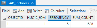
- Use the Summary Statistics (or Frequency) tool to tally the number of times (i.e., the count) that a GAP cover type occurs in the table for each separate HUC. Include the sum of the
Countfield in your analysis; this will be useful in the next step when we calculate species density.
Examine the output table. The resulting table should have a row for each HUC and a column (FREQUENCY) indicating the number of different GAP habitat types found within it as well as the total # of cells in the planning unit. The FREQUENCY column therefore lists the planning unit’s richness! You should find that the HUC12 with the ID of 1 has 5 separate cover types and 1588 total pixels of habitat in it.
- Use the Alter Field tool to rename the
FREQUENCYfield toRichness
2B. Data visualization
ArcMap offers a quick and easy way to display these results as an interactive histogram…
-
First, we need to join the summary status result table to back to a raster or vector dataset of HUCs. To do this, make a copy of the HUC12 raster (to preserve the initial raster, in case we make a mistake), and join the summary stats
RICHNESSfield to it using the Join Field tool. This allows you to display your HUCs by its species (i.e GAP cover type) richness. -
Create a histogram of the results, by right-clicking the raster layer to which you just joined the summary stats and selecting
Create chart>Histogram. Set it to use 10 bins. Then, with both your raster layer and histogram visible, click on one of the histogram bins; you will notice that the corresponding HUC12s are selected – a nice exploratory feature of graphs in ArcMap.
NOTE: An alternative, easier way to do all these steps is to perform a zonal variety analysis with the HUCs as zones and the GAP land cover as the values. However, this doesn’t give us the HUC_GAP table that is useful in further analyses…
2C. Estimating evenness from GAP cover data
Say we have two HUCs, both having 10 different GAP cover types. They will have identical richness values, but one HUC may consist of 95% of a single cover type whereas another has roughly equal representations of all 10. We may want to favor the latter as it actually gives us a more rounded distribution of cover types.
To get at this, we need to calculate evenness, for which there are a few indices. We’ll calculate the Shannon’s diversity index which measures the relative abundance or proportion of individuals among all species found within a HUC:
Shannon’s Index ($H’$) reflects both the richness and evenness of species within an ecosystem (here, a HUC12 planning unit). The proportion of a species $i$ in a given HUC relative to the number of species ($_i$) in that HUC is calculated and then multiplied by the natural logarithm of this proportion ($ln (P_i)$). The resulting product is summed across all species in the HUC and multiplied by -1.
$H’ = - Σ (P_i* ln(P_i)) $
The first step in calculating the Shannon index is to calculate the set of $P$ values – the proportions of each cover type within a given HUC. We derive this number as the area (i.e., the cell count) of a given GAP cover type divided by the area (cell count) of the HUC in which it’s found. The area of a cover type found in a HUC is listed in the attribute table of the HUC_GAP raster (the result of combining the HUC12s and GAP cover types - see the first part of Step “A” above). If we add a column to this attribute table that lists the total area (i.e. cell count) of the HUC, we can easily calculate $P_i$ by dividing the two numbers. And we can add the column of HUC area by joining the attribute table of the original HUC raster.
-
Use the Join Field tool to join the
Countfield from the HUC12 raster to the HUC_GAP attribute table.TIPS:
- The Join Field tool can be flaky when working with raster attribute tables. If you have issues getting your join to work, try converting your
HUC12raster attribute table to stand alone tables using the Copy Rows tool, then joining that product to yourHUC_GAPattribute table. This does not seem to be an issue with the current version of ArcGIS Pro. - Be sure to use the appropriate field in the
HUC_GAP; it’s not the VALUE field…) - If you re-run your “Join Field” tool, you will continue to add more fields to your HUC_GAP attribute table. You may wish to delete those fields if they appear, or you can simply re-run the Combine tool used to create the dataset.
- The Join Field tool can be flaky when working with raster attribute tables. If you have issues getting your join to work, try converting your
Take a look at the updated HUC_GAP attribute table. It still includes a field listing the HUC ID (HUC12_90M, the GAP cover type found in that HUC (AZ_LANDCOVER), and the amount of that GAP cover type (COUNT), but it now has a second “COUNT” field (it’s field name is actually (COUNT_1) that lists the total area (in cells) of the HUC. The snip shown below lists the values for cover type 36 (“Colorado Plateau Pinyon-Juniper Woodland “) found in HUC 131:
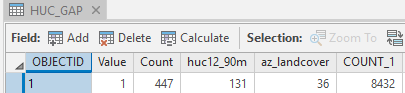
It indicates that there are 447 pixels of cover type 36 found in HUC 131. And since HUC 131contains a total of 8432 pixels, this means that cover type 36 comprises $447/8432$ , or 5.3% of the HUC’s area. This is this HUC-GAP type’s $P_i$ value.
The remaining steps include adding a column to calculate $P*ln(P_i)$ for all HUC-GAP type combinations. We could do this incrementally by creating a column to hold the $P$ values (equal to [Count] / [Count_1]), then another column to hold $ln(P)$ (equal to Log([p])), and a finally third column calculated as -1 * p * ln(p), but we can do calculations easily in one step…
- Add a field to the HUC_GAP attribute table. Name it
P_lnPand set its type to “Float”.
Since $P_i$ = the area of the HUC’s (COUNT_1) field divided by the area of GAP cover type i in the HUC (COUNT), then we calculate $P_i$ * ln($P_i$) using the following Raster Calculator equation:
P * ln(P) = -1 * (!COUNT! / !COUNT_1!) * math.log(!COUNT! / !COUNT_1!)
We now have a list of $P_i$ * ln($P_i$) values for each GAP cover types in each HUC. We’ll now sum these values for each HUC to get $\Sigma(P_i * ln(P_i))$ portion of the Shannon Index calculation. (You could divide these values by $H_(max)$, which would be $ln(S)$ where $S$ is the total number of GAP classes in the landscape, but since we are interested in relative values, not absolute values, this is not necessary…)
-
Use the Summary Statistics tool to calculate the sum of all the
P_lnPvalues calculated above for each habitat HUC (i.e., by using theHUC12_90mas the case field). You should find that the HUC12 with the ID of 1 has a Shannon's index value of 0.199.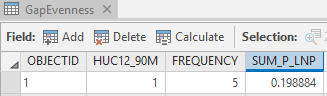
The resulting table contains the Shannon Diversity index for each HUC. The higher the values represent more diverse HUCs. To display these data on a map, we could join this table to our HUC raster and symbolize the data using the Sum_P_lnP values.
There are additional diversity indices that we might want to consider – ones that emphasize rare habitat types or HUCs that, though perhaps not diverse, contain the only instance of a species/habitat type. Most of these additional diversity indices begin with the same table as these two, namely a list of the HUCs, the GAP habitats they include, and their relative proportions within the HUC. After that, analysis is often easier when done using other software, and so it makes little sense to include in this exercise. Instead, let’s now look at alternatives to the GAP classes for calculating diversity.
3. Creating biophysical “zip-codes”
In cases where GAP or similar classified habitat data either don’t exists, are inadequate, or are at an inappropriate scale for analysis, we can attempt to create our own surrogate datasets to derive estimates of species diversity across a landscape. These methods can be useful, but are certainly quick and dirty and should be used with care and error checked, if at all possible.
The surrogate dataset we’ll create here is based on a few biophysical characteristics of a landscape known to correlate with biodiversity fairly well in mountainous regions, namely temperature, soil moisture, and solar exposure. Each of these we can derive from a DEM, which is quite useful given that DEM data are quite ubiquitous. Temperature is highly correlated with elevation via adiabatic lapse rates. Soil moisture values can be obtained from soils data, if available, or from a topographic convergence index layer derived from the DEM as we did in previous labs. Solar exposure can also be derived from the DEM via the hillshade method, also done in a previous lab.
These three data layers, all containing continuous values, are classified into a few discrete breaks and then combined together into a raster layer of unique “Zip-code” combinations of elevation class, TCI class, and solar exposure class. Each zipcode is considered to be a unique ecological zone, so once we’ve made our zipcode map, we can use the same techniques to calculate richness, evenness, etc. as we did above.
The zip-codes that are made depend quite a bit on where the breaks occur. A method we’re developing here at the Nicholas School involves finding natural breaks in elevation, TCI, etc. using whatever species observation data (e.g. Natural Heritage Element Occurrence (NHEO) data, or Global Biodiversity Information Facility (GBIF) point observation). We will use BISON plant element occurrence data to determine breaks in our zipcode breaks using the steps outlined below.
3A. Steps to Create Zip Codes for the Mogollon Plateau
-
Create a copy of the BISON plant element occurrence shapefile. We are about to modify the attributes and it would be good to do this on a copy instead of the original in case a mistake is made.
-
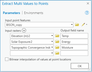
Use the Extract Multi Values to Points tool to extract values from the Elevation, Solar Exposure, and Topographic Convergence rasters for each point in the BISON\_plant features. This will add three new columns to the feature class listing the elevation, TCI, and solar exposure at each plant location.
Examine the attribute table of the resulting feature class. Are there any null values in the fields we just created? If so (and there should be), we’ll need to remove them as they may skew our subsequent analysis.
- Use the Select tool to extract into a new feature class only those point features produced above that don’t have any null values in the last three columns. (You should now have 17,908 remaining point features.)
Now we need to find natural breaks within the range of values of elevation, TCI, and solar exposure. We can do this via the symbology settings for the BISON_plant (copied and non-null) features.
- Open up the symbology for the feature class and select Graduated colors under the Symbology section. Set the Value field to be Elevation and classify the values into 5 classes using natural breaks.
- ►►Important: click on the Advanced Symbol Options (
 , at the top of the symbology panel) and expand the
 Sample Sizeoption. The default sample size is 10,000, but we have over 18,000 points. So to use all our samples, we’ll need to increase this: set the Maximum sample size to100,000. ◄◄
From the classification window you can view the histogram of values and the natural breaks within the values:
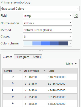
This gives us the break we want to use to divide elevation/temperature into classes. Record these numbers.
Find the natural breaks for the solar exposure/energy and TCI/moisture values as you did above to fill out the remainder of the table.
| Class | Temperature | Energy | Moisture |
|---|---|---|---|
| 1 | 1889 | ||
| 2 | 2156 | ||
| 3 | 2498 | ||
| 4 | 3149 | ||
| 5 | 3806 |
Next we reclassify the values in the elevation, insolation, and TCI rasters using these breaks. For elevation we will create a raster using all 5 class values. For insolation and TCI, however, we want to emphasize the upper and lower extremes and lump the middle three classes together. Note that the break for the 5th class is different than that which is shown in the figure. This value should be set as the highest value in the elevation dataset so that all cells are included.
-
Reclassify each of the Elevation, TCI, and Solar Exposure raster layers 5 classes using the breaks informed by the plant locations.
-
However, for the final break, be sure you use the maximum value of the raster dataset (e.g. 3847 for Elevation).

-
For the TCI and Solar Exposure datasets, set the 2nd, 3rd, and 4th classes to be classed into the same values (e.g., 1,2,2,2,3). We are less certain about these breaks and by grouping the middle three of the five classes, we are only separating out the extremes.
-
We’re left with 5 temperature (elevation) classes, 3 soil moisture (TCI) classes, and 3 solar exposure classes – or a total of 45 potential zip-codes – which we can use as an alternative surrogate dataset to estimate HUC diversity. (Note: you may not actually have all 45 classes; some combinations may not be present in your dataset.)
- Combine the three classes made in the previous step into a single zipcode dataset.
→ Calculate HUC richness, density, and Shannon diversity index values for each HUC based on the zip-codes they contain using the methods in the earlier part of this lab.
Summary
After completing this and the previous three lab exercises, we now have calculated several HUC attributes on which to base a prioritization of HUCs for protection. Our next exercise will examine various ways in which these attributes can be combined to find the overall best suite of HUCs to select based on different conservation objectives.
►Deliverables◄
- Compile the following into a single Word document named
<netID>_BiodiversityLab.docxand submit the document onto Canvas. Do NOT submit your ArcGIS workspace.
GAP species richness
-
Histogram of species richness across HUC 12 planning units – 10 bins (as described in lab).
-
Identify the HUC(s) with the highest GAP species richness value. (If more than one HUC has the highest richness value, include the IDs of all the HUCs with this value. Include both the HUC id(s) and the richness value.
GAP species evenness
-
A histogram of the Shannon’s Index ($H’$) values across HUC 12 planning units – 20 bins.
-
Identify the HUC(s) with the highest Shannon’s Index value in terms of GAP cover types. Include both the HUC id(s) and the index value.
Biophysical ZIP-code development
- Submit a table of the breaks used to create the temperature class map, the soil moisture class maps, and the solar exposure class map from the elevation, TCI, and solar exposure datasets, respectively. Screen grabs of the reclassification tables used in your models are fine here...
Biophysical Zip-code richness
- Identify the HUC(s) with the highest species richness in terms of biophysical zip-codes. (If more than one HUC has the highest richness value, include all IDs of all HUCs with this value. Include both the HUC id(s) and the richness value.
Biophysical Zip-code evenness
- Identify the HUC(s) with the highest Shannon’s Index value in terms of biophysical zip-codes. Include both the HUC id(s) and the index value.