Lab 6: Conservation Planning - Optimization with Marxan

Correction from the recordings…
In looking at the Marxan output (e.g at the 10:50 mark of recording 5), I point out numbers (e.g. Value, Cost, PUs) for the initial state of the Marxan iteration, not the optimized result.
. Instead, I should be pointing out the last line in the iteration’s report.
This shouldn’t have any major impact on the rest of the lesson, particularly because we get the correct information when looking at the output files (vs the report screen).
Introduction
Materials/Data
Analysis Steps
Overview
A. Preparation for Analysis
B. Creating hexagon planning units
C. Adding cost and status values to the planning units
D. Adding species representation values
E. Running the ArcMarxan tools
F. Editing the spec.dat file
G. Setting MARXAN run-time parameters
H. Running MARXAN
I. Reviewing conservation target representation in the optimal solution
J. Mapping the planning units included in the MARXAN solution
Assignment
Introduction
We’ve spent the past few weeks developing landscape attributes that can be used to rank, sort, and prioritize our Mogollon planning units (HUC 12s) for conservation. The next step is to establish a method to combine all these metrics into a decision support system (DSS) that land managers can use to evaluate different land use scenarios (i.e. different prioritization schemes) and identify which set of HUC12s make up the most efficient combination given a specific conservation objective.
Sorting. The simplest means to do this (especially from a GIS standpoint) is just to sort the HUCs on one or a few of the landscape attributes we’ve developed. For example, take the top X% of the HUCs in terms of, say, pronghorn habitat area, and then from those, take the top Y% of HUCs in terms of low threat, etc., until you have a predetermined area of [quality] pronghorn habitat or species conserved – or until you have run out of funds.
A second, slightly more complex approach is performing a weighted overlay of the various HUC attributes, much like we did in creating our weighted threat classification a few weeks back. From there, we sort the HUCs on their overall score and select enough HUCS until an objective is met.
These two methods can be quite useful, but they don’t necessarily achieve the most parsimonious solution. They both employ a purely “greedy” algorithm meaning that each HUC is selected for its ranking, independent of what’s already been selected. It’s possible that the two top ranked HUCs may each have the highest richness scores. However, if most of the species included in HUC 2 also occur in HUC 1, you might get a better overall richness score if you chose HUC 1 and a HUC ranked lower than HUC 2 if it included more species that were not included in HUC 1. In short, you may want to look for the set of HUCs that most complement each other.
Using previous selections to inform subsequent ones is known as a heuristic approach, i.e. one that learns as it goes. A greedy heuristic approach does exactly what is mentioned above: finds the single best HUC and then adds another HUC based on how it complements already selected ones. However, this approach also may not achieve the most parsimonious solution. It could be that a starting with a combination of two lower-ranked HUCs rather than the single top ranked HUC leads to a more efficient overall suite of HUCs.
So, it turns out that finding the exact combination of HUCs that ends up with the single most parsimonious suite of HUCs is not that easy! It involves evaluating every unique combination of HUCs. With our 142 HUCs, that would be $2^{142}$ or roughly $10^{42}$ combinations!!
So instead, we use an approach called simulated annealing to poke around for optimal solutions. This approach uses something of a greedy heuristic approach, but uses a “cooling factor” whereby sub-optimal HUCs are occasionally added to the portfolio to explore whether they may ultimately lead to an overall more parsimonious solution. To do this we use Marxan…
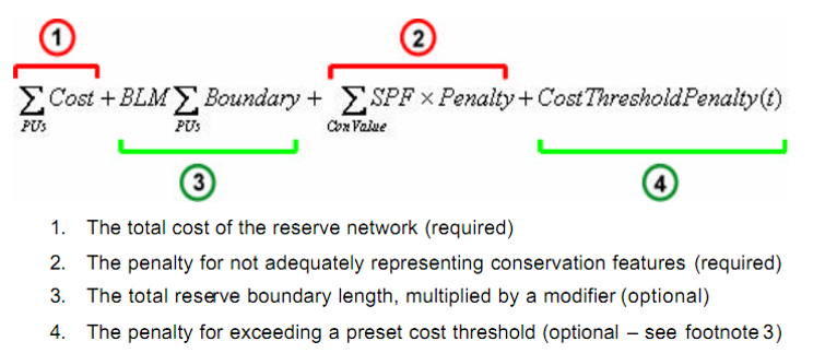
Marxan is a standalone program that allows the user to identify suites of planning units (i.e. patches or HUCs) that maximizes conservation goals with the least amount of cost. Marxan attempts to find the optimal suite using the simulated annealing process. The process starts with seed HUCs (either randomly selected or user defined), and then adds other HUCs at random, each time evaluating the marginal gain or loss of adding that HUC using an objective function which is based on the cost of adding the HUC and the contribution to meeting a specified target. The HUC is added to the portfolio if its gain exceeds a threshold ($T$). At first, the threshold is set low – allowing more sub-optimal HUCs to be included in the ongoing portfolio. But as more HUCs are added the threshold increases, and thus only HUCs more likely to contribute to an overall solution are added.
Marxan is may not find the single most optimal solution. Instead, it makes several repeat runs from the same inputs and points to the best solution of those runs to be our optimal solution. En route to this, Marxan also produces a listing of how frequently each HUC occurs in the optimized solution from each run (called the “summed solutions”). Both are useful in arriving at a conservation portfolio.
In this lab, we explore how Marxan is applied to our Mogollon datasets. We use ArcGIS to create the Marxan input files and then run Marxan. Both the “best solution” from 100 model iterations and the “summed solution” are displayed geographically using ArcGIS. It is not intended to be an exhaustive review of Marxan and what it can do, but it should give you enough familiarity with the software to explore further and also some idea on how to create the inputs from familiar datasets using ArcGIS.
Materials/Data
For this exercise, you’ll be given (in the OptimizationLab.zip file). This file includes:
-
The familiar set of Mogollon data and study area boundaries.
-
The Arizona Gap Analysis Program land cover dataset, clipped to the study area.
-
The HUC12s (raster and vector) with attribute tables that includes each of the patch/HUC metrics that we have calculated over the past several weeks. (Note that these are slightly different values than many of those you have calculated, so don’t be tempted to use these values to check other lab exercises…)
-
A modified version of Apropos Systems’ ArcMarxan Toolkit. More about this toolkit is described below. The tool provided in your workspace has been updated (here at Duke) to work with ArcGIS Pro. [If needed later, this modified version can be obtained here: right click on the ‘raw’ link and save the
.pytfile.]
Analysis Steps
Overview
Marxan requires 5 input files to run. These files contain necessary information on the planning units (pu.dat), the conservation targets (spec.dat), the amount of conservation target found in each planning unit (puvsp.dat), the amount of shared or exposed boundaries among planning units (bound.dat), and finally run-time options for Marxan execution (input.dat). (Refer to the Marxan documentation for a full description of these files.)
These files are simply text files, but they adhere to a specific format; deviating from that format will prevent Marxan from running, and often with little clue why it’s refusing to run. Fortunately, the ArcMarxan toolkit takes care of setting up a proper Marxan workspace and configures all these files. Still, we need to generate the GIS file from which ArcMarxan creates these files. And we also need to devise models that can process the Marxan Outputs.
And so the workflow include the following:
- Prepare our workspace
- Identify and prepare our planning unit features
- Assign costs to each planning unit feature
- Set the status of each planning unit feature
- Compute the how much each conservation feature is represented in each planning unit
- From these data, generate the Marxan workspace and files.
- Adjust species representation goals.
- Run Marxan
- Map the results
- Adjust Marxan run-time parameters and examine the change in results
A. Preparation for analysis
- Download the lab data (OptimizationLab.zip) to your local drive and expand it.
You should see a formatted workspace that includes the datasets mentioned above along with a folder named Software. This workspace contains the Marxan executable (Marxan_x64.exe), the Inedit.exe program, and two folders: MarxanInputs and MarxanOutputs. The workspace also contains the ArcMarxan.pyt Python toolkit modified to work with ArcGIS Pro.
B. Creating hexagon planning units
While we’ll be using the HUC12s as planning units, it’s good to know how to construct tessellated planning units as well. Below are the steps for this:
- Use the Generate Tessellation tool, setting the extent and spatial reference equal to the Mogollon Plateau boundary shapefile. For this exercise, a 10 sq km hexagon should be an adequate size.
This generates hexagons for the entire extent of the provided feature class. However, we want to remove those falling completely outside the study area. We can do this by using the Select Features By Location tool to select features intersecting the Mogollon Plateau feature class, but then we should write the selected features to a new feature class so that the remaining features have sequential feature IDs, which will streamline bookkeeping later on.
- Select features intersecting the Mogollon Plateau.
- Copy those selected features to a new feature class.
Lastly, while the internal feature id (FID or OBJECTID field, depending on whether you saved as a shapefile or geodatabase feature class) is sequential, it’s never good to rely on those values remaining consistent; ESRI internal IDs can change without notice, so we’ll want to save these values to a new field.
- Create a new field called
PU_idand calculate them as equal to the internal ID. If the first internal ID value is zero, add one to the values so that IDs begin with 1.
C. Adding cost and status values to the planning units
We need to assign cost and status to attributes to each planning unit. We’ll go back to using our HUC12s, but make a copy of the HUC12 feature class (to have a pristine backup) and use the copy for the following analyses.
The cost field refers to the cost of including a given planning unit in the reserve, and is used by Marxan to find the least costly portfolio of units meeting our GAP cover representation objective. Costs can be actual dollar amounts to acquire the unit, if known, but more often a proxy of cost is used. Common proxies are unit area (the larger the unit the more costly to acquire) or perhaps area within a certain ownership class (e.g. private land could be more expensive than public land). However, unit costs can include anything that favors one HUC over another, including opportunity costs such as the cost of not including a HUC that has good metrics.
In our example, however, we’ll keep it simple for now and just use the area field: the cost of a HUC will simply be the area of the HUC, in acres.
- Add a field to the planning unit feature class called
Cost - Set values equal to the area of the planning unit feature (i.e., its
shape_areavalue)
The status field is used to specify any HUCs that we might want to ‘lock’ into or out of the final solution – regardless of whether it contributes to the optimal solution. This can be in cases where we know that one or a few HUCs will already be protected and we want to find the other HUCs that will complement these best. We’ll begin our analyses setting all values in the status field to zero indicating that none are locked into or out of the final solution.
- Add a field to the planning unit feature class called
Status. - Compute all status values have a default value of
0.
We can seed our Marxan runs to start with a set of planning units by setting the status of those PUs to 1. We’ll favor betweenness centrality in our analysis by setting the PUs with the top 10 betweenness centrality scores to have a status of 1. (Alternatively, we could lock those PUs in by setting the value to 2.)
-
Open the attribute table of the planning unit feature class (the copy, that is).
-
Sort the values in descending order on the
BetweennessCentralityattribute. -
Select the top 10 rows.
-
Update the status values to
1.
D. Adding species representation values
The next step is to add a column to our PU feature class for each conservation feature we want to include in our reserve portfolio and in that column list the amount of that conservation feature that is represented in the PU. If you had raster datasets of species abundance or density for individual species you could compute these values using zonal statistics and then join the appropriate values to the planning unit attribute table.
In our case, however, we are going to use GAP cover types as proxies for species and design a reserve network that contains representative amounts of each cover type. Therefore, rather than single rasters for each conservation target, we have one raster that includes all conservation target. This actually makes our job easier as we can use the Tabulate Area tool quickly generate a table listing the area of each GAP cover type falling within each planning unit.
- Run the Tabulate Area tool to generate a listing of how much each GAP cover type occurs within the planning unit features.
- Join this table to your planning unit feature class containing the
CostandStatusfields created above. - Do not include the following files in the Join Fields list:
A_,Agriculture,Barren_Lands__Non_Specific,Developed__Open_space__LowIntensity,ObjectID_1,Open_Water, andRecently_Burned. (Note: There’s a short cut to adding many fields at once in the Join Field tool: it’s the icon just to the right of the Join Fields label…)
Take a quick look at your PU attribute table to ensure everything looks ok.
E. Running the ArcMarxan Tools
With the PU’s tagged with a cost, status, and conservation target areas, we now have what we need to use the ArcMarxan tools to generate the Marxan inputs.
First we need to create a folder for our Marxan data.
- Create a sub-folder named
HUC12in the Software folder in your workspace.
Next, we use the ArcMarxan Create Input File and Folders tool to create the Marxan workspace
- Run Create Input File and Folders, selecting the
Pronghornfolder we just created as the project folder. - Inspect the folder in Windows Explorer to see what the tool created.
Create the Marxan files using the following tools. For each, use your PU file and the input folder created above as the tool inputs. Select the other tool inputs appropriately.
- Use Export Planning Units File to create the
pu.datfile - Use Export Feature Files to generate the
spec.datandpuvsp.datfiles. Be sure to select all your conservation features to yourFeature fieldsinputs! - Use Export Boundary File to create the
bound.datfile.
Examine the output files in a text editor.
F. Editing the spec.dat file
The default spec.dat does not include proper representation targets for our conservation features. We will edit it in Excel, setting default targets of 30% of the existing extent of each.
- Open a new blank MS Excel document.
- Click and drag the spec.dat onto this document. (This opens the file in Excel making for easy editing…)
- Change all values in the
propcolumn to0.3. - Change all values in the
targetcolumn to-1. This enables us to override target values with percentages in thepropcolumn. - Change the species penalty factor (
spf) values from1to1000. A higher SPF will make MARXAN work harder to get every species’ target met in the final solution. - Save the document in its current format (csv). Excel will complain “Some features in your workbook…” Disregard and choose
Yes. Then close Excel, opting not to save. (We just saved!)
G. Setting MARXAN run-time parameters
With our input tables set, we’re now ready to set the run-time parameters for our MARXAN analysis. The Inedit.exe program (found in the Software folder) is used to create and modify the “input.dat” file that contains the run-time settings read by MARXAN when executed.
-
Copy the Inedit.exe program into your
HUC12scenario folder (the one containing the “input”, “output”, and “pu” folders). -
Open up this copied Inedit.exe program.
-
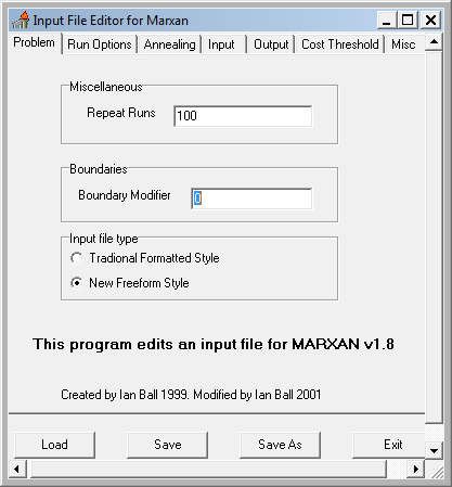
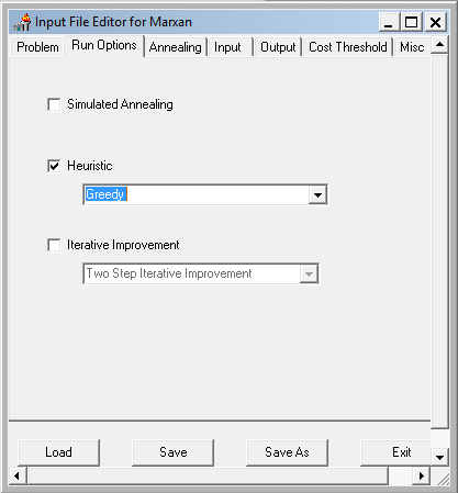
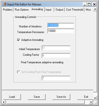
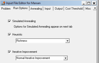
Configure the settings to match the screen captures below. This initial setting will run a purely greedy richness algorithm, i.e. no annealing. Later we’ll modify this to use simulated annealing and see if it finds a more cost efficient solution. Note: make sure to set the input and output paths to where your data files are!
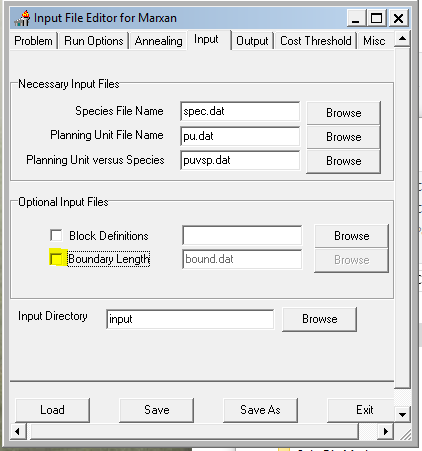
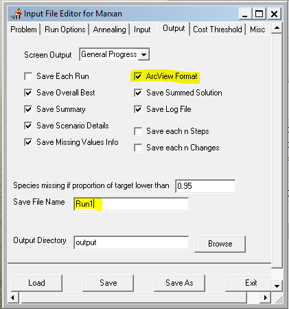
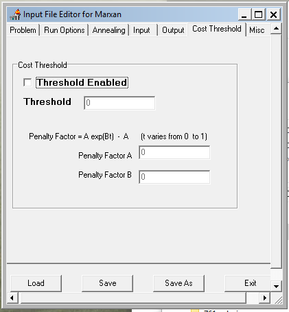
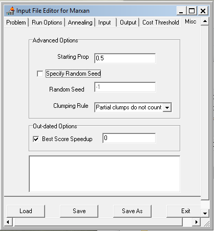
- Save and exit the Input Editor.
TIP: Set the random seed to 10 to get the same values I provide, otherwise your values will be different…
H. Running Marxan
- Copy the
Marxan_x64.exefile from thesoftwarefolder into yourHUC12folder. - Double click the copied
Marxan_x64.exefile to run Marxan. A black DOS window should appear and scroll through various computations as the program runs. If it hangs, you likely have an error in one of your input files and you’ll have to do some detective work to find out where the errors is…
When Marxan completes, it will have created 5 new files in the MarxanOutput folder. These files, each named after the string you provided in the “Save File Name” entry in the Inedit.exe program above, include:
- A summary file listing the results of each run (“
_sum.txt”) - A table listing in how may runs was each HUC included in the optimal portfolio (“
_ssoln.txt”) - A listing of each of the planning units included in the single most optimal solution found (“
_best.txt”) - A listing of each conservation feature (GAP type) & how it fared in the best solution (“
_mvbest.txt”) - A summary of the model run and the parameters used (“
_sen.dat”)
The Marxan documentation contains full explanations of each of these files, but we’ll take a quick look at three of these file and use two of them, the “_best.txt” file and the “_ssoln.txt” files, to display our results in ArcMap.
I. Reviewing conservation target representation in the optimal solution
The _mvbest.txt file created by Marxan (in your output folder) lists all the conservation targets (i.e. the GAP cover types) and summarizes how each fared in the best solution found by Marxan.
- Open the _mvbest.txt file in a text editor, or better yet, rename the extension from .txt to .csv and open the file in Excel. This file lists all the conservation targets (i.e. the GAP cover types) and summarizes how each fared in the best solution found by Marxan.
→ The last column indicated whether the target was met or not. Were any targets missed?
J. Mapping the planning units included the Marxan solutions
Of the 100 iterations Marxan runs, the solution with the lowest objective function score bubbles up as the “best solution”. The planning units (i.e. HUCs) included in this solution are listed in the _best.txt output file. This file can be joined with the HUC dataset to map out these HUCs.
Marxan also provides another useful result: the summed solutions files. This file, _ssoln.txt, lists each HUC and the number of times that HUC was included in the solution of a particular iteration. We ran 100 iterations of the HUC selection process, so a value of 99 for a given HUC (for example) in this table indicates that the HUC appeared in all but one of the solutions.
This metric is useful as it identifies HUCs that may not appear in the single “best” solution, but occur frequently in sub-optimal solutions. There must be some reason why this HUC keeps on getting selected, and this allows us to see that.
Use the steps below to map out the HUCs involved in the single best solution as well as to display the frequency that each HUC occurs in the solution set of all Marxan iterations.
- Create a new layer of your HUC12_UTM feature class in your map.
- Join the
_best.txtand_ssoln.txttables to the HUC12_UTM features. If you have any trouble joining these text files to your polygon layer, you might want to convert the text files to proper ArcGIS tables (either in a geodatabase or as DBF files) before joining.
You can now display HUC polygons as those occurring in the single best solution of all runs, or labeled by the number of times each appears in the optimal solution in a single run.
Assignment
This assignment will not be a formal lab report. Instead, we will Marxan a few times with our HUCs with different run time settings to explore the different ways in which optimization can be calculated.
A. Complete the following Marxan runs, being sure to rename output so that the files are not overwritten.
-
Run 1: Greedy heuristic (this is the one we just did above).
-
Run 2: Simulated Annealing coupled with a *Richness* Heuristic AND using Normal Iterative Improvement. (Simply check Simulated Annealing, set the Heuristic to “Richness” and the Iterative Improvement box in the “Run Options” and select Normal Iterative Improvement.)
-
Run 3: Same as Run 2, but this time we’ll include a boundary length modifier to focus in on a reserve that also favors connectivity. To do this, set the Boundary Modifier (Problem tab) to 0.5, set the Boundary Length file (Input tab) to bound.csv (if not already), and check the box next to it. Doing this adds a new cost to the objective function that relates to the overall amount of edge in the output reserved design: a more compact set of HUCs will be favored.
-
Run 4: Same as Run 3 , but this time, rather than seed the top 10 HUCs in terms of pronghorn betweenness centrality, lock in these 10 HUCs so that they are ensured to be in the final portfolio. (Hint: See page 46 in the MARXAN manual, located in the Docs folder in your ArcGIS project workspace.)
B. Examine the results of the above runs and fill out the missing values in the MarxanResults.xls table.
Values for the first three rows of the MarxanResults.xls table (in the Docs folder) can be obtained by looking at the _sum.txt file generated for each run. Open the table in ArcGIS and sort on the Score column, from smallest to largest. The row with the lowest score represents the ‘best’ solution. Use the values in this row to identify the total cost, the number of planning units, and the number of missing targets in the best solution and fill out the corresponding rows in the MarxanResults.xls table.
Add the _ssoln.txt file to ArcMap. This file, which lists in how many iterations of Marxan analyses did a particular planning unit appear in the solution (max = 100), contains the information you need to figure out the remaining two rows in the MarxanResults.xls table.
C. Create simple maps showing the HUCs in the best solution for Runs 2 and 4.
Include only the Mogollon Plateau boundary and the HUCs in this map. No other cartographic elements are needed; this map will not be scored on elegance, but the reader should be able to easily discern included HUCs from excluded ones (i.e., make included HUCs dark and excluded ones light).
D. Create simple maps showing HUC frequency in the solutions for Runs 2 and 4 (i.e, use the ssoln.txt files).
Set the break values in the symbology to show HUCs that occur in 0, 25, 50, 99, and 100 solutions of the 100 model iterations. Don’t worry if some classes have no HUCs or if HUCs are too small to show in your map.
► Submit your two sets of maps, your
MarxanResults.xlstable, and a brief interpretation of the results listed in the MarxanResults.xls table. Include in your summary the following:
- Why to do the best runs in each of the 4 scenarios differ in cost? In number of planning units?
- Why might some runs have fewer planning units but higher costs?
Also, zip up your entire Software folder and submit it to Canvas.