Habitat Modeling Project - Part 1: Preparation and background
Contents
- Step 1.1. Preparing your workspace
- Step 1.2. Compile information on the species (ecological model)
- Step 1.3. Generate a list of environmental variables (data model)
- Step 1.4. Build a geodatabase of relevant environmental variables
Step 1.1. Preparing your workspace
- Create a workspace using the standard format we’ve been using (project folder with
Data,Docs,Scratch, andScriptssubfolders, etc.). - Extract the contents of the SDM_Exercise.zip file (on Canvas;l you may need to log in to get access to the file) and move contents to the appropriate directories. (MaxEnt files can go either in the root folder or the Scripts subfolder.)
- Create a new ArcGIS Pro project document. Add the toolbox provided in the zip file as well.
Step 1.2. Compile information on the species (ecological model...)
The first step in any habitat modeling exercise is to become as familiar as you can with the species you are modeling. In the framework presented by M.P. Austin (2002), this constitutes our ecological model. This model helps guide the analysis and likely make your work more efficient and productive. There are a few useful sites for finding general information, and even some distribution data, for species. These include:
-
NatureServe Explorer: https://explorer.natureserve.org/Taxon/ELEMENT_GLOBAL.2.844117/Desmognathus_wrighti
-
Crespi, et al (2003): http://onlinelibrary.wiley.com/doi/10.1046/j.1365-294X.2003.01797.x/pdf
-
Animal Diversity Web: https://animaldiversity.org/accounts/Desmognathus_wrighti/
From these sources, you can determine the following information about the pigmy salamander…
-
It’s usually observed between 1600 and 2012 m in elevation, but has been seen as low as 762 m.
-
It’s often found near spruce fir stands at higher elevations, and mesophytic cove forests at lower elevations.
-
While it’s entirely terrestrial, 76% of the observations were within 61 m of streams.
-
It hides under moss, leaf litter, logs, bark, and rocks.
-
It hibernates in underground seepages.
-
There may be two distinct populations, one northern and one southern
Note: AI Chat Bots can be of use here, if used judiciously. Ideally, we’d want to involve true experts on the species we are modeling, but instead we are relying on a web search, which may or may not be accurate or complete. Similarly, an AI response may not be accurate or complete, but the search is certainly faster! And some ChatBots like Perplexity provide resources. Here’s a link to my search - LINK; we can discuss the differences in class.
Step 1.3. Generate a list of [possibly] relevant environmental variables (data model…)
So, with this background, we can generate a more informed hypothesis about our species. For example, we see that elevation is important (though we can only speculate why: temperature?). Furthermore, we have some general vegetation associations to narrow in on, and we see that moisture is important as the salamander needs seepages for hibernation. We are not aware of any direct relationships with the solar exposure or slope, though those factors may have important indirect contributions to temperature. There may well be other factors, but our first-hand information is limited.
The ensuing step is to generate our data model, i.e. to see what spatial data sets we might have or could generate that could serve as proxies for the above conditions. Elevation is an obvious one. Rainfall and temperature means and fluctuations may also prove useful. A vegetation map of the thematic resolution that identities the classes important to a salamander, if available, would be another useful data set. For the moisture constraints, we aren’t likely to have a map of underground seepages, but perhaps a soils map or one of our DEM based moisture maps could prove useful. (Yes, we are simplifying things a bit here, but for the purposes of the exercise, this should be fine…)
Step 1.4. Build a geodatabase of [possibly] relevant environmental variables
It’s here where we apply the skills developed in the previous class sections to assemble a geospatial database to develop proxies for the environmental conditions outlined above. In the first section (as well as in previous GIS courses), we reviewed a number of techniques for locating and obtaining many of these datasets. However, we’ll use this opportunity to review some additional techniques, ones that tap into the vast number of datasets available as services on ESRI’s Living Atlas and ArcGIS online. We also examine how the model builder and other tools (Python scripts) can be used to automate and document this process.
The sections below walk you through the process to download, subset, and project several datasets we’ll use in our analysis. In some cases - those marked by the ![]() - I have provided you with the geoprocessing models used generate the rasters used, both to save a bit of time and also to demonstrate new concepts. In others, you will have to build the models yourself.
- I have provided you with the geoprocessing models used generate the rasters used, both to save a bit of time and also to demonstrate new concepts. In others, you will have to build the models yourself.
In the end you want the following datasets
1.4.1 Elevation 
Exploring an elevation “imagery layer” service
We will extract elevation data from ESRI’s “Ground Surface Elevation - 30m” imagery layer. Before extracting the data, let’s explore it and better understand how image service layers differ from familiar raster datasets.
-
Have a look at the Item Page for this service and explore its properties.
- Note what the page suggests for appropriate usage of the dataset (e.g. visualization vs analysis)
- Note the list of “Server Functions”; we’ll discuss those shortly.
- Note the source of the data and its native coordinate system and resolution.
- Finally, note the analysis restriction of a 24,000 x 24,000 pixel limit.
-
Let’s add the service to our map:
- Find the URL for this service and copy it to your clipboard.
- In ArcGIS Pro, with your map active, select
Add Data>From Pathand paste the URL. - Zoom to the extent of the dataset.
→ We now have elevation data for all of North America added to our map!
-
Explore those Server Functions:
- Set the elevation service as the active layer in your map and select the Data item in the top menu.
- From the
Processing Templatesdropdown select one of the options, e.g.Hillshade.
→ The imagery service includes not only elevation data but algorithms to compute and visualize elevation derivatives!
-
Explore some other capabilities…
- Set the
Processing Templateback toNone(raw elevation) - From the
Create Chartdropdown, selectSurface Profile. - Use the tool to create an elevation profile for a small segment. (Don’t go too large, as it may take a bit of time!)
- Set the
-
Remove the service from your project. (We’ll add it again via a geoprocessing tool.)
Extracting data from the imagery service
Getting back to our project, the Ground Service Elevation imagery layer includes the 30m elevation dataset we want for our modeling exercise. I’ve created a geoprocessing model that connects to the imagery layer service, extracts the data we want from it, and wrangles it into a projection system, extent, and cell size we will use in our analysis. You’ll find this in the SDM_DataPrep toolbox as the 1. Elevation Service Extraction model.
- Open the model in edit mode.
- Note the first process:
Make Image Service Layer. Open this step and examine the inputs.- What are the primary inputs and outputs?
- How is the Analysis Mask used
- Can we alter the tool to produce rasters not of elevation, but of derivatives like slope, aspect, hillshade?
- Run the tool and zoom to the extent.
- Do you still get data for all of North America?
- Run the remaining tools in the model to project and clip the dataset.
- Why do you think we subset the image service data when we are going to just clip it later?
The result should be an elevation raster, projected to the same coordinate system as the analysis mask, and clipped/snapped to the extent of the analysis mask.
1.4.2 Land Cover (NLCD & GAP)
Next we want to extract land cover data to use as inputs to our model. Similar to elevation, we’ll tap into imagery layers hosted on online. The NLCD raster is part of the Living Atlas, and another land cover dataset, one with more vegetation categories, come from the US Gap Analysis Project (GAP), hosted on ArcGIS Online. Again, we will use the opportunity to explore these imagery layer service before extracting data from them for our model.
Time-enabled Imagery Layer Services: National Land Cover Dataset (NLCD)
- In the Catalog Pane, search for USA NLCD Land Cover and add the result to your map.
- With the layer selected, click on the layer in the map to reveal information at for the pixel you clicked. You’ll see that you queried not just one but many layers. The NLCD imagery layer is not just one, but a collection of imagery datasets.
- You may also see a time slider in your map, which allows you to subset time slices and even animate change over time.
- And yes, this imagery layer also has its own processing templates. Explore those.
- When done playing, remove the NLCD imagery layer from your project.
Extracting Land Cover (NLCD & GAP) for our model
- Open the
2. Land Cover Service Extractionmodel in theSDM_DataPreptoolbox. - Notice the Expression parameter in the
Make Image Service Layertool associated with the NLCD Land Cover Service.- What do you think we are we selecting there?
- Which processing template are we using?
- Where might you find more information on this imagery service?
- Examine the same tool associated with the GAP Land Cover imagery service.
- Anything worth exploring with this dataset?
- Run the model, setting the outputs to go to
EnvVars.gdbgeodatabase.
At completion, you should now have the 2006 NLCD and the US GAP land cover layers, respectively, added to your maps with each layer projected to the same coordinate system and extent as the Analysis Mask as well; just like with the elevation dataset.
1.4.3 Climate Data (PRISM)
Oregon State’s PRISM Climate Group provides access to its “30-Year Normals” datasets which include average monthly temperature and precipitation assimilated from over the past 30 years. Unlike the previous datasets, these are not provided as services, but the monthly normals can be downloaded, which I have done via their download page.
Downloading the data
I selected the 800m resolution data and downloaded “All Normals Data (.bil format)” for Precipitation, Mean Temperature, Min Temperature, and Max Temperature. The resulting zip files were expanded into their own folders, found on the W: drive in the 761_data/PRISM/data folder. Each folder contains 13 raster datasets in BIL format: one for each month and an annual one.
Variables to process
For our habitat model, we want to summarize each PRISM variable to generate climate means and “extremes” across the dataset’s 30 year history. The products we want to derive include: mean monthly precipitation, precipitation of the driest month and of the wettest month, as well as mean minimum monthly temperature and mean maximum monthly temperature
-
PPT_mean: Mean monthly precipitation - Mean pixel value across all 12 monthly precipitation rasters. -
PPT_min: Rainfall of the driest month - Minimum pixel value across all 12 monthly precipitation rasters. -
PPT_max: Rainfall of the wettest month - Maximum pixel value across all 12 monthly precipitation rasters. -
TMEAN_mean: Mean monthly temperature - Mean pixel value across all 12 monthly TMEAN rasters -
TMEAN_min: Coldest Monthly Temperature - Min pixel value across all 12 monthly TMEAN rasters. -
TMAX_mean: Warmest Monthly Temperature - Max pixel value across all 12 monthly TMEAN rasters.
Processing the data - Python
In the PRISM folder, you will also note a subfolder named code which contains Python code I used to process these datasets. While the dataset operations outlined above could be done in a geoprocessing model, coding the task in Python is much more robust and actually quite a bit faster. You can view the code in the read-only HTML document. Or you, by double clicking the Jupyter Notebook link, you can explore and execute the code. You are welcome to ask questions in class on this, but we won’t be covering Python in this class.
The product of this code is a geodatabase - PRISM_data.gdb - containing summaries of each of the PRISM monthly rasters. Each projected and clipped to the Analysis Extent raster, as was done with the other datasets.
1.4.4 The
EnvVars.gdbgeodatabaseLater in this lab, we are going to export all the environmental variable rasters into a format that statistical analysis software can read. This process will be explained later, but a step we can do now that will facilitate that process is to place all these raster products into a single geodatabase. Here are the steps to do this:
- Create a new geodatabase named
EnvVars.gdbin your project workspace.- Create a new geoprocessing model in your project toolbox called
1. Run Data Extraction Models.- Add the three geoprocessing models in the
SDM_DataPrep.atbxtoolbox to this geoprocessing model created above.
- For the first two models, ensure the Analysis Mask input is set to the Analysis Mask raster. And set the outputs to be produced in the
EnvVars.gdbgeodatabase. Name theseElevation,USA_GAP_LandCover, andUSA_NLCD_2006, respectively.- For the third, ensure the
Prism_data.gdbinput points toW:\761_data\Project3_Data\PRISM\data\PRISM_data.gdb(where the processed PRISM data live), and theEnvVars.gdbpoints to the geodatabase created above.- Run all the models. It may take some time, but in the end you should have 9 rasters in your
EnvVars.gdbgeodatabase.Next, we’ll move on to adding more environmental variable rasters derived from these and other datasets.
1.4.5 DEM derivatives
While we could use the processing templates included with the Ground Surface Elevation imagery layer to derive slope, aspect, and hillshade, I find it’s a bit faster to run these processes on our already clipped and projected dataset. We’ll also create a few more DEM derivatives, so we might was well create our own local geoprocessing tool for this. Here, you’ll also see that a number of terrain-based tools we developed in the last model have since been adopted as their own built-in ESRI models!
All the products except the
Aspect_30andHillshade_30should go into yourEnvVars.gdbgeodatabase;
Aspect_30andHillshade_30can go into the Scratch.gdb geodatabase.
- Create a new geoprocessing model in your project’s toolbox named “
2. Surface Analysis” - Compute slope as percent rise using the
Surface Parameterstool:-
SlopePct_30: Neighborhood = 30 m, Percent Rise
-
- Compute aspect using the
Surface Parameterstool:-
Aspect_30: Neighborhood distance = 30m
-
- Compute northness and eastness from the aspect30 product using the Raster Calculator:
-
Northness=Cos("%Aspect_30%" * math.pi/180) -
Eastness=Sin("%Aspect_30%" * math.pi/180)
-
- Compute topographic position using the
Multiscale Surface Differencetool:-
TPI_250: Min = 30m; Max = 250m; Increment = 30m -
TPI_2000: Min = 1500; Max = 2000; Increment = 100m
-
- Compute shaded relief/insolation using the
Hillshadetool:-
Hillshade_30: Azimuth = 315; Altitude = 45 -
Insolation_30: Azimuth = 225; Altitude = 30; Model shadows
-
- Compute topographic convergence using the “
Calculate TCI” script tool provided in the “SDM_DataPrep” toolbox provided.-
TCI_30: [using Elevation as the input]
-
1.4.6 Distance to stream
Next, we want to investigate whether distance to stream is a good predictor of salamander habitat. The end product, Dist_to_stream should go into the EnvVars.gdb geodatabase.
- Create a new geoprocessing model to compute this layer; call it ‘3.
Hydrologic Analysis’ - Create a stream raster using the “
Derive Stream As Raster” tool, using an accumulation threshold of 900,000 sq m (1000 30x30m cells). -
Dist_to_stream: Compute Euclidean (planar) distance to the stream pixels created above using theDistance Accumulationtool.
1.4.7 Forest density
Finally, we want to explore whether the density of nearby forest might correlate with the presence of salamanders. Without know what “nearby” means precisely, we’ll try two different values: amount of forest within 150m and within 400m.
To do this, we’ll extract “forest” pixels from the US GAP land cover dataset, defining forest as: “Central and Southern Appalachian Northern Hardwood Forest” (class 63); “Southern and Central Appalachian Oak Forest” (class 84); and “Central and Southern Appalachian Spruce-Fir Forest” (class 96). Then we’ll use focal statistics to determine the proportion of these forest types within 150m and 400m, respectively:
- Create a new geoprocessing model to compute forest density; call it ‘
4. Forest Density Analysis’ - Use the
Test(orCon) tool to create a binary raster of forest/non-forest, where forest is specified as USA GAP Land Cover classes 63, 84, or 96. - Add two instances of the Focal Statistics tool to compute the following, with the products going into the
EnvVars.gdbgeodatabase.-
FocForest_150: Mean value for pixels within a 150m radius. -
FocForest_400: Mean value for pixels within a 400m radius.
-
You should now have 19 raster datasets representing your environmental layers all in a single folder. That folder should look like this in ArcCatalog (though your names may be different):
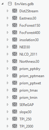
Furthermore, each of these rasters should have the same extent and cell size as the Analysis mask. If you open up the properties of each and click on the Source tab, they should show they have 3187 columns and 3051 rows in the Raster Information setting.
Once these rasters are created, we are ready to begin map the salamander’s habitat using an arsenal of rule based and/or statistical approaches.