Project - Albertine Rift Pipeline Analysis (Part 1)

Scenario
The African Conservation Organization (ACO) has just learned that the government of Uganda plans to construct a new pipeline to deliver oil from a central processing facility south of Murchison Falls National Park to a refinery in the Kabale parish in Hoima, Uganda. Two potential routes have been proposed for the pipeline, and a hearing on the two options is being held in a few weeks. This is the ACO’s only opportunity to voice any concerns about the biological impacts of each proposed route and present their recommendations.
The ACO has reached out to you to help evaluate the impacts of each proposed route on people, forests, and streams and suggest which route is best. They have been provided with a shapefile of the proposed pipelines, but with very little documentation. Also, the ACO has no available data on land cover, population, and hydrography so you will have to find what you can via public domain sources.
Once you have located and prepared the necessary spatial data, you’ll need to determine for each route:
- The estimated number of people within 2.5 km of the proposed route.
- The total area (km2) of wetlands within 2.5 km of the proposed pipeline route.
- The total length in which the pipeline travels through an established protected area (km)
The best route will have the least area of wetland, the fewest people in the impact zone (2.5 km buffer), and will cross the fewest streams. Compile your findings and present a memo to the ACO with your recommendation based on your findings. Be sure to support your findings with effective maps.
Learning Objectives
- Gathering and organizing spatial data for a specific objective (data portals & data formats)
- Defining projections when projection information is missing
- Proper naming and symbolizing of data layers
- Geospatial analysis in the ArcGIS model builder
- Interpreting and communicating results
 Recording Updates
We noticed the following discrepancies/updates between the recordings and the lab documents
- 1.0 - Overview: Ignore the dates on “What’s next” at the end of the recording.
- 1.3 - Getting Population Data: The site hosting the GRUMP data has indeed changed (as warned in the recording). I redirects to https://www.earthdata.nasa.gov/centers/sedac-daac. From there, log in, search for GRUMP, and in the results, find “Global Rural-Urban Mapping Project, Version 1 (GRUMPv1): Population Count Grid” and go to the Direct Download link.
- 1.6 - Analysis: The values presented in the recording are INCORRECT. Consult the PPT or the results shown at the end of this document for the correct ones.
If you happen to find any other discrepancies, please let me know and I will update them here.
Getting to work…
The analytical objectives here are pretty clear, but where you might find the data to do the analysis is not. In lecture, we have discussed some public domain datasets you might explore. You can also search some useful data clearinghouses like ArcGIS online and DataBasin.org. First, however, we should take inventory of what we have been given and get an idea of the region and spatial extent we are concerned with. So, we’ll begin by creating a workspace and preparing the data the ACO has provided.
1. Set up a project workspace
As mentioned in last week’s exercise, the first step in most any analysis is to create a workspace for your project. The steps below follow those same steps we did in that previous exercise.
- Create the project workspace folder in your V: drive. We’ll call it “ACO_Pipeline”.
- Create the
data,scratch, andscriptsfolders as subfolders in this project workspace. - Open ArcGIS Pro and select
Create a new project. Set the project name name toACO_Pipelineand store it the folder you just created drive, making sureCreate new folder for this projectis not checked. - Set your workspace environment settings to point the project’s default workspace and scratch workspace to the
ACO_Pipeline.gdbandscratch.gdbgeodatabases, respectively. (Analysis->Environments). - Create a
README.txtfile and add a short project description as well as your name (or email), and the date.
2. Add and prepare provided data
You are provided three shapefiles in the MurchisonPipeline.zip file. The first, Endpoints.shp, includes where the pipeline will start and end, namely the processing facility south of Murchison Falls and the refinery in Kabale parish. This dataset has a defined projection: UTM Zone 36 North, WGS 1984. However, the two pipeline route shapefiles do not, and we are left to guess what projection these files are in. We can never be certain that we’ll get the correct projection, but with some good detective work, we can sometimes become reasonably sure we got it.
-
Unzip the contents of the
MurchisonPipeline.zipfile into yourDatafolder. -
Create a new map and add the
EndPoints.shpshapefile to your map. - Add
Route1.shpto your map. Based on your knowledge of this dataset, it should appear as a line connecting the two points in theEndPoints.shpfeature class above. However, nothing appears!? - Suspecting a projection issue with the data, examine what coordinate system to which the
Route1.shpfeature class is referenced. You’ll see it’s not defined. Furthermore, no documentation exists suggesting what coordinate system the data should be defined as. *We’ll have to guess!
Determining the projection of dataset with no defined coordinate system
To figure out what coordinate system our data should be in, we alter our map view’s coordinate system until our problematic layer appears where it should be. (Layers with known coordinate systems will reproject on the fly.) And since we our EndPoints dataset has a defined coordinate system, we’ll know we are correct when the ends of the Route1 layer lines up with it.
First, we'll need to know our map view's current coordinate system.
Open up the properties of the Map view and check it’s coordinate system. Make note whether this is a geographic or projected coordinate system, i.e. whether it uses spherical or Cartesian units.
Next, we can deduce whether our dataset uses a geographic or projected coordinate system by seeing how it's displayed on relative to our known map coordinate system.
Zoom to extent of the feature layer in question and look at both the scale and coordinate values shown at the bottom of the map view’s window. Do these values make sense given the current projection? If they are absurd, e.g. the scale is super large or super small, then your mystery dataset likely uses the opposite type of coordinate system (PCS vs GCS) than the map. That is our first clue and narrows down which coordinate system our datasets uses – a bit.
What remains is guessing what the likely coordinate system is.
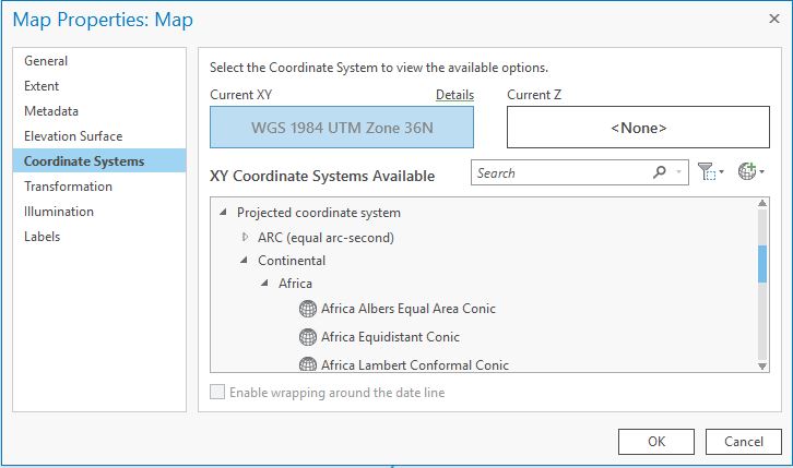
Change the coordinate system of your map view window (via the Map’s properties). The
EndPoints.shplayer added to our map has a defined projection. This enables ArcGIS Pro to reproject these features on the fly. OurRoute1.shpfeature class has no defined projection, so ArcGIS will not attempt to reproject it; the features will assume the coordinates use whatever coordinate system the map uses. This allows us to guess at the coordinate system and see if we are right; if we are right, our feature will align with other features of known projections. So, let the guessing begin.Open the map’s properties and select the
Coordinate Systemstab. We know we have a projected coordinate system from looking at the layer’s coordinates (above), so expand theProjected Coordinate Systemssection. We still have a lot of options to choose from, and any information you can glean from your data source will be helpful in narrowing the choices. Unfortunately, we have nothing to go on – but we do know our dataset is in Africa. Let’s expand Continental and select Africa:→ Try
Africa Albers Equal Area Conicand select OK. You may have to zoom to theRoute1layer. It appears close, but not quite dead on it since the start and end should match the points in theEndPointslayer.→ Go back to the map’s properties and try
Africa Equidistant Conic. How do the line features in theRoute1layer match up now? Looks like we have a winner! Sometimes this method of guessing at an undefined projection is all you can do to use the data. It can be handy, but it comes with some risk – you may have arrived at what looks to be the correct coordinate system, but actually isn’t (e.g. NAD 27 and NAD 83 based systems are very close, but not exactly the same). It’s always useful to try to find documentation on the data’s coordinate system. But when you just need to move on, you should ALWAYS acknowledge that you guessed at the coordinate system when submitting your result.
- Now, add
Route2.shpto your map. This dataset also has no defined coordinate system. See if you can figure it out and then project this dataset to match theEndpoints.shpfeature class too. If you get too stuck, ask an instructor, a TA, or a fellow student to see how they found it (and try to figure out how they got it and you didn’t) – but don’t waste an inordinate amount of time guessing.
At the end of this step, you should now have a proper workspace with three feature classes with properly defined coordinate systems. We’ve not created any new datasets .
3. Searching for data
Like finding the correct coordinate system for a dataset with limited or no metadata, searching for data is also something of a wild goose chase. There’s no correct way to locate the exact data you might need. Rather, you need familiarity with what datasets might be out there, awareness of useful up-to-date data portals, and a strategy for general web searches. Your search can take a variety of directions. You may want to begin by looking for what datasets might be available for the geographic region of your analysis (e.g. “Albertine Rift” or “Uganda”). Or, you may want to start by looking for data by theme (e.g. “wetlands”, “protected areas”). Again, there’s no correct answer and, unfortunately, there’s a degree of luck involved.
Here, we’ll begin our search for data together. It’s quite possible you’ll find a more recent, more accurate, more precise dataset on your own, and if you do feel free to use it in your analysis. Recall, however, that we have a limited budget to get our work done in this case, so you need to get the feel for when your continued data search starts to be more effort than its worth. With that in mind, let’s dive in! First, we’ll review what public domain datasets might be useful, and then we’ll scout out some of the more promising geospatial portals.
♦ Public Domain Datasets
In lecture, we reviewed several public domain datasets that may be useful here. Most of these (i.e. the non-US ones) were global, so we know our study extent would be included. The questions we then have to ask are: are these data resolute enough (spatially and thematically) to serve our purpose? Are they recent enough? Sifting through these would be a good place to start, and we’ll go ahead and tackle our first dataset – population – using the public domain dataset of population provided by SEDAC, i.e. the Global Rural-Urban Mapping Project, or GRUMP (v1).
Download and prepare the GPW dataset for Uganda
- Start at SEDAC’s main web page: http://sedac.ciesin.columbia.edu/
- Register/log in to the site (required to download data).
- Find the link to browse their data collections and find GRUMPv1.
[ You will see a link to download the more recent GRUMPv4, but we’ll stick with v1 for this exercise…]
 - Decide whether population count or population density is more appropriate.
-
Download the dataset for Uganda. Data for the year 2000 is the most recent, so use that.
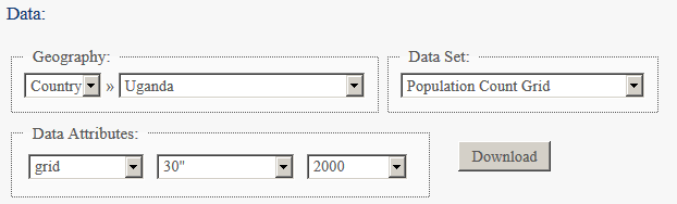
- Add the data to your map. You may see that two versions of the data are provided. Be sure you understand the difference among the two and how that might affect your results.
![]() For consistency sake, use the
For consistency sake, use the ugaup00ag (i.e. the "adjusted") dataset.
►Note that it’s not always clear cut and rarely are two download sites ever the same. You need to learn how to navigate these sites. And yes, sometimes you need to make an account and log on before you can download the data you want…
►Also, keep in mind potential bias a data provider might have along with other limitations of the data. Remember: if you don’t have a firm grasp of the analog data on which a digital dataset is based, you may be providing your client with a misleading result.
►If you are unable to locate the dataset to download, a direct link is here.
♦ On-line spatial data platforms
As you’ve just seen, SEDAC provides many more datasets than just the GRUMP population data. It’s useful to take note of that, i.e. add it to your mental or physical list of sites to visit when searching for useful or relevant datasets. Now, however, we’ll turn our attention to on-line resources whose purpose extends beyond just hosting spatial data and more into allowing users to search across a broad spectrum of data providers for specific datasets. We’ll examine two of the most useful data platforms currently available: ArcGIS Online and Data Basin.
ArcGIS Online
Recognizing that finding data is a challenge, ESRI has made significant efforts to facilitate data discovery. These efforts are always evolving, but with ArcGIS Pro ESRI has integrated a powerful data search utility directly within it desktop application – though the same catalog is available on-line via a web-browser. This is referred to as ArcGIS Online, and can be hugely help in searching for data. To access the service from within ArcGIS, activate the Catalog frame and select the Portal tab. Finally, select the All Portal “cloud” icon so we search the entire ArcGIS Catalog collection.
Searching for data with ArcGIS Online can be done by topic, by geography, or sometimes both. We’ll see how ArcGIS Online can help us find a good wetlands dataset for our analysis.
-
Try first to search for a good wetlands dataset by using “wetlands” as your search term. If you see any potentially useful datasets, you can click the details box for more details. One important attribute to note is the type of data being shared, e.g. map service, web map service (WMS), feature service, layer package, etc. These dictate how you can use the data in your analysis: some types of data can only be viewed in your map while others allow you to perform analyses with the features.
►Did you find any useful wetlands datasets by searching globally for “wetlands”? Try adding one or a few to your map. Open up the dataset’s properties in ArcMap. What can you tell about the dataset? Was anything saved to your computer? Where?
-
Next, try adding a geographic search term. Type in “Albertine Rift” as a keyword. Too narrow perhaps? Let’s broaden it; try “Uganda”. Scroll down to see if there are any useful wetland datasets in the search results. Or, you could search for “Uganda wetlands”.
-
To further filter your results, we can include only certain item types. Set your search to:
Uganda wetlands type:feature. If that fails, then perhapsUganda wetlands type:package. -
Find and add a few promising wetland datasets to your map. Investigate the datasets: are they raster or vector data? Can you add the dataset to a geoprocessing model?
![]() For consistency sake, search for
For consistency sake, search for Uganda wetlands type:package and add the Wetlands extent and types for Uganda - 1996 (Data Basin Dataset) result to your map.
- Note where the dataset is saved. Is it in your project workspace? If not, consider copying (and perhaps re-projecting) the dataset into your data folder…
Data Basin
Data Basin (http://databasin.org/) is another excellent resource for finding spatial data. You may have actually found a wetlands dataset via ArcGIS Online that was hosted at Data Basin! We’ll use Data Basin to search for a dataset of protected areas in the Albertine Rift area. Before searching, however, you should register yourself with Data Basin. It’s free and it’s required to download many datasets from the site.
Once you are registered and log in, search for protected areas in Uganda. Again, you could begin your search by theme (“protected areas”), by geography (“Albertine Rift”, “Murchison Falls”, “Uganda”), or both.
Once you’ve executed your search, the results can take many forms. Some returns may be downloadable datasets, some may just be maps (or map services that you can display on-line or sometimes in ArcGIS), and others may be documents or figures. You can also sort your results by relevance, by name, or creation date.
![]() For consistency sake, let’s select the Uganda protected areas dataset provided by the Conservation Biology Institute for our exercise:
For consistency sake, let’s select the Uganda protected areas dataset provided by the Conservation Biology Institute for our exercise:
http://databasin.org/datasets/c5ef5cca827a42de87f7bce418e52bcb
At this page, you’ll see it’s available both as a Layer Package and a Zip Archive. Both can easily be displayed and used in ArcGIS; we’ll go with the Layer Package.
Download the zipped layer package file to your Data folder and uncompress it. You can add the .lpk file directly to your map and it will appear as a symbolized feature class. You now have all the data necessary to complete your assigned task! We are ready to move onto the next step – preparing the data for analysis.
4. Prepare your data
Once you’ve found and obtained the data required to do your analysis, you may still want or need to prepare the data for analysis. Like the pipeline route data, you may need to define the dataset’s coordinate system and also project the data to match the coordinate system of your other datasets. Depending on the analysis, you may also want to convert vector data to raster, or if it’s already raster data, resample the data so that the cell size matches other datasets. You may also want to create spatial subsets of datasets that extend far beyond your area of interest so that your workspace consumes disk space more efficiently.
The exact preparations needed in a given situation depend on the requirements of your analysis and the format of other datasets. What you should do each time, however, is keep a log of any significant changes you’ve made to the original data. This is best done by updating the metadata attached to these datasets. However, if you modified the data using a geoprocessing model, you could also refer to that model as a clear guide to what changes you’ve made to the data in preparation for analysis.
Note: Sometimes you shouldn’t project raster data!
While it’s generally good practice to get all data into a single coordinate reference system, in our case you will not want to reproject the population raster to match the other vector datasets. Why? Because when we reproject a raster, we resample the actual rasters, i.e., we alter the data. This is true with vector data as well, but to a much lesser extent. Thus, when we perform analyses that mix raster and vector datasets, it’s always best to reproject the vector to conform to the rasters coordinate system, not vice-versa.
Why then don’t we reproject all the vector data to match the coordinate system of the one population raster? That’s because the population raster uses a geographic coordinate system, meaning all distances are measured in spherical units (degrees). This make computing distances and areas awkward, so we are better off keeping the vectors in a projected coordinate system – unless we need to use them in an analysis that involves the raster.
Ahh, projections…
For consistency sake:
- Project all your vector data to the same coordinate system as the
Route1.shpfeature class (Africa Equidistant Conic).- Keep the population raster in its native WGS 84 geographic coordinate system.
- Set your map’s coordinate system to that of
Route 1as well.- When projecting, do NOT select the option to preserve shape.
Tidy your prepped data & document your work
Tidying your data
Once your data are prepped and projected, it’s wise to take a moment and tidy your project. Geospatial analysis is confusing enough as it is, so pausing to keep things organized is a good habit to form. This can be as simple as renaming and symbolizing your layers to clarify the data elements you are working with:
- Explore custom symbols that add more meaning and clarity to your points, lines, and polygons.
- Play with the transparency of layers.
- Set custom breaks in raster layers, and round values to places that reflect the precision of your data.
- If your raster data have continuous, not categorical values, set the resampling type to bilinear in the raster display properties.
Documenting your work
You invested time in preparing the layers for analysis. Consider saving these steps in a Geoprocessing model. This may be quite useful if, for whatever reason, you have to redo your work. It’s also an important step in being transparent about your work and making it fully reproducible.
A few tips on this:
- View your analysis history by selecting History with the Analysis menu active.
- Add the elements in the history to a new geoprocessing model; your model should be complete in no time!
- However, take a moment to tidy up the model elements. Could you understand exactly what you did if you returned after, say, 6 months?
5. Execute your analysis
Now that we have the data required to perform our analysis, the next step is, of course, to execute the analysis. In this case, the analysis is relatively straightforward: you simply need to calculate the values of the three questions asked for the two pipeline scenarios. The actual values you get, however, may vary depending on the datasets you chose, and it’s your responsibility to be as transparent as possible regarding any decisions you made that may affect the results.
I strongly suggest that you perform all your analysis by building a geoprocessing model. This is useful for at least two important reasons. First, it provides an excellent outline of your analysis that can be reviewed and perhaps revised later if needed. Also, since our analysis is repetitive (same steps for two different pipeline routes), you can just update the pipeline feature class and rerun your model to get your results!
Some notes on processing your data:
- “Buffer” or “Pairwise Buffer” - Both do the same thing, but “Pairwise buffer” is faster. Ask in class if you don’t know why. Results *should* be exactly the same regardless of which tool you use, but they are NOT.
- If presented with an option to use “Planar” or “Geodesic”, choose Planar. If you were doing this professionally, you’d chose Geodesic, but Planar is faster in this case. Don’t know the difference between these? Ask in class…
- Likewise, if you are reprojecting vector data and are given the option to “Preserve Shape”, your results will be more accurate, but in the scheme of things, the increased accuracy won’t make a huge difference, so leave this option un-checked.
- The results I get in the recording for the area of wetlands and length of pipeline in protected areas are WRONG. (I used a incorrectly projected Route 1 feature class
.) The correct values are below.
6. Present your results
We will revisit different ways in which you can present your results later, but for now do your best at answering the questions asked, restated here for convenience:
For each pipeline route, provide the following:
→The values you should get for Route 1 are provided - with full precision - to check your work… NOTE THESE ARE DIFFERENT THAN WHAT’S IN THE RECORDING.
| Layer | Amount (full reported precision) |
|---|---|
| The estimated number of people within 2.5 km of the proposed route 1 | 36,941.022168 people |
| The total area (km2) of wetlands within 2.5 km of the proposed pipeline route. | 53,568,320.82920693 sq m |
| The total length in which the pipeline travels through an established protected area (km) | 43,426.745764 m |
Additional checks:
| Layer | Amount (full reported precision) |
|---|---|
| Route 1 (Africa Equidistant Conic) - Full length | 109,303.582618 m |
| Route 1 Buffered 2.5 km - Area | 56,3621,029.26107 sq m |
| Route 2 (Africa Equidistant Conic) - Full length | 111,941.502972 m |
Deliverables
When you have completed your analysis, tidy up your workspace (e.g. remove any temporary files, and update documentation where necessary) and compile your results in a short document that you’d submit to the African Conservation Organization. (Note: you’ll have an opportunity to revise this, but time invested in preparing this as best you can may well pay off…)
Summary/What’s next
At the end of this exercise, you should have more confidence in your ability to find data to perform a specific geospatial analysis. You should also have a keener appreciation that finding data is not always an easy or straightforward task, but that with some basic knowledge of general public domain datasets, some key on-line data platforms, and some search know-how, you can learn to become more efficient and more successful in your search for valuable geospatial data.
While in future lab exercises in this class, the data will be provided for the most part, you will likely need to search for data at some point – your course project for example. In Part 2 of this lab, we’ll continue with this project, discussing more about how communicating your results can be nearly as important as knowing how to produce the results in the first place.