Project 2 - Sierra Costera Site Evaluation (Part 3)

Overview - Part 3
In this lab, we continue our examination of terrain and ecohydrology in the Sierra Costera de Oaxaca. We did the bulk of the analysis in the previous lab, but there are a few additional useful techniques relating to processing DEMs to go over.
Learning Objectives
| Section | Objectives |
|---|---|
| 6. Creating Watershed-Based Planning Units | • Explain the utility of watershed based planning units • Adjust stream detail with different flow accumulation thresholds • Use the Stream Link tool to split streams into segments• Create planning units via the Watershed tool and Stream Link outputs |
| 7. Identifying Riparian Areas | • Explain the utility of identifying riparian areas • Create an adjusted flow direction raster to allow measuring distance TO streams • Use the Flow Length tool to measure distance to stream |
| 8. Identifying Floodplains | • Create “watersheds” where values are the elevation of the cell into which it drains • Compute vertical distance between cell & stream from the above result. |
The Flow Distance Tool |
• Invoke the Flow Distance tool to replicate the riparian and flood plain results above. |
Recordings
- Proj 2.3 - Watershed Planning Units (14:20)
- Proj 2.3 - Identify riparian areas (23:21)
- Proj 2.3 - Identify floodplains (25:13)
6. Creating Watershed-Based Planning Units
This course deals a lot with prioritizing landscapes for action; we seldom have the resources to protect an entire landscape, so we have to identify subsets of the area where we can focus our efforts. To do this, we need to divide the landscape into planning units. Based on several factors, a planning unit is either included or excluded in the set of area we tag for conservation, but however we make those decisions, we still need to devise a useful way to divide the landscape into these units.
Watersheds, basins, catchments, hydrologic units – whatever you want to call them – often provide an excellent means for dividing a landscape into planning units. They are scalable. They follow somewhat natural, ecologically meaningful boundaries, and they are relatively easy to create using a DEM.
In the previous lab, we reviewed how to delimit the drainage area for specific pour points. In this exercise we review a procedure used to parse the entire landscape into watershed planning units. It requires a Flow Direction and Flow Accumulation raster, both easily derived from a DEM as seen in the previous lab, and the Stream Link tool.
The process goes as follows (which you should do in a new geoprocessing model):
-
First we generate a new stream layer, similar to as we did before, i.e., by setting cells below a certain flow accumulation threshold to no data and the rest as a single value. Create your stream raster using a [D8] flow accumulation threshold of 2000 cells, (i.e. cells with a flow accumulation less than 2000 will not be considered a stream; those with an accumulation of 2000 or more will).
-
Then, use the Stream Link tool to assign unique identifiers to each branch of this stream raster.
Have a look at the resulting raster and be sure you understand what’s going on.
-
Finally, create watersheds using your Stream Link product as the pour points. Yes, it creates a catchment for each stream pixel, but as the pixels along a specific branch have the same value, the upstream catchment is assigned the same value and they essentially merge into a common zone!
→ You should get
364unique planning units in your output raster… (NOTE: This is different than the values computed in the recording.) -
(Optional) You may wish to convert these planning units to polygon features.
You now have a dataset you can use to prioritize your landscape. Each watershed planning unit can be assigned various attributes, and based on these attributes prioritized for inclusion in your final conservation plan – a topic we will revisit later in this course.
What would you change to create more (but smaller) planning units or fewer (but larger) ones? Are all the watershed planning units valid, i.e. hydrologically correct, watersheds?
7. Identifying Riparian Areas
The land immediately adjacent to streams often has special value for conservation. For one, natural vegetation in the riparian zone can act to buffer pollutants such as excess nutrients and sediments generated upslope that would normally flow directly into stream courses. Intact riparian zones can also provide natural corridors linking habitats for many species.
Mapping riparian zones is often done simply by buffering stream features a set distance. This can be done either with the Buffer tool, if using vector stream features, or the Euclidean Distance tool, if working with rasters (or vectors). This procedure provides reasonable approximations of riparian area, but it neglects the fact that water does not travel “as the crow flies” but rather follows the terrain until it spills into the nearest stream.
The following steps outline the procedure for using ArcMap’s Flow Length tool to [somewhat] easily calculate distance from stream along the flow path, which can ultimately provide a more accurate estimation of riparian zones. The Flow Length tool calculates distances along the flow path, and it does so in one of two directions: upstream and downstream. Upstream flow length tags each cell with the distance to the furthest upstream pixel. This can be useful for computing hydrographs, but it’s not all that useful to us. Instead, we are interested in downstream flow length which tags each cell with the distance (along the flow path) until a NoData cell is reached.
The Flow Length tool itself is fairly straightforward, but there are a few tricks to getting it to do exactly what we want. First of all, we want to calculate flow distance to the nearest stream, not to the watershed outlet. To do this, we need to set all stream cells to NoData before calculating flow length. And once we’ve calculated that, it’s likely we want to add the stream cells back into the result, which may sound easy, but it can be somewhat confusing with all the switching between Data and NoData values it requires.
Anyway, here are the steps.
-
Create a new geoprocessing model to calculate riparian area via the Flow Length method.
-
First we want to create a FlowDirection raster where all the stream cells are set to NoData so that we can calculate flow length to the nearest stream, not the watershed outlet.
- Add the 90m Flow Direction and Flow Accumulation rasters (D8) you created in the previous lab.
- Using the SetNull tool, set all cells with a
flow accumulation >= 300(i.e. stream cells) toNoData, setting the values of the remaining pixels to the Flow Direction raster.
Take a look at the output. It should look exactly like the original flow direction raster, except that stream cells are now set to NoData. -
Add the Flow Length tool to your model. Set it to use the modified flow direction raster you just created and keep direction set to
Downstream.The output is nearly what you want, but you’ll note that the stream cells are still set to NoData. Also, these distances do not account for travel through the cell itself (you can see that all cells adjacent to a stream have a flow length of zero). We need to apply two adjustments… -
Using the Plus tool, add 45 (1/2 the cell size of 90m) to all values in the output of your Flow Length process. This adjusts the flow length from the edge of the cell to the center of the cell.
-
Finally, to add the stream back to the result, we’ll again use the original Flow Accumulation raster to identify stream cells: if a cell is a stream, we’ll set the value to zero, otherwise we’ll set the value to be the adjusted flow length we create in the previous step. You can do this with the Con tool.
We are left with a raster where each cell is the distance along the flow path to the nearest stream. This dataset has a variety of uses. We can select cells up to a given distance threshold to identify riparian corridor. We can also use it to identify how far non-point source polluting cells are from streams as a way of spatially adjusting their potential impact on stream water quality. Baker et al (2005) provides an excellent overview of how Flow Length and land cover rasters can be used to greatly improve estimates of non-point source pollution impacts on streams.
8. Identifying Floodplains
Another useful dataset is one that shows floodplains, or the area adjacent to a stream that’s likely to get flooded if the streamflow were to exceed a certain depth. Here we will examine a procedure for creating a raster showing all the pixels that are no more than 2m above the cell into which it drains. Then we will examine some useful derivatives from this dataset.
The key in creating this dataset is to create an elevation layer where values are not relative to sea level, but rather to the stream in which the cell drains. We do this by assigning elevation values (as integers) to the stream cells and then using these as pour point values for the watershed tool. Subtract this result from the actual elevation, and we have relative elevation! There’s one catch, however. A 2m difference in elevation is a pretty fine measurement to extract from a 90 m DEM, so we will only do this analysis using the 15m DEM.
Here are the steps to execute this analysis:
- Create a new geoprocessing model to calculate floodplain area.
- Before calculating the elevation difference between upslope area and stream, we’ll need a stream raster. If you haven’t created one from your 15m dataset, create one now. (Use a 1000 cell flow accumulation threshold.)
- If your DEM is a floating point raster, the next step would be to convert these floating points to integers so that elevation values can be used as pour point locations in the Watershed tool. If your terrain is relatively flat, you may want to multiply values by 10 or 100 to maintain subtle changes in elevation before converting to integer (e.g. an elevation of 10.483 m would be come 105 cm). Note that our 15m DEM is already an integer raster so there's no need to do this step.
- Now you need to extract these integer DEM values for just the stream cells. You can use the Extract by Mask tool (or Con or SetNull…) to do this. These will become your pour points for the next step. Yes, there are gobs of pour points and two adjacent stream cells may have the same value. That’s actually ok!
- Next, use the Watershed tool to create watersheds for all these elevation pour point pixels. Examine the result and be sure you understand what the output cell values represent (and how it became that). As the instructor or a TA if you are not entirely clear.
- To compute the elevation relative to the stream (vs sea level) we subtract watershed tool output from the original DEM. In doing so, we are left with the difference between the actual elevation of a pixel (in m above sea level) and the elevation of the stream pixel into which the pixel drains!
- Lastly, isolate all the pixels in the above result that are less than or equal 2. This output is your 2m floodplain. With this dataset you can characterize by the proportion of area within the floodplain.
Breaking Update! A new tool!!
ESRI has recently added a new tool to their toolbox: Flow Distance. This tool greatly simplifies both processes of defining areas within a specific flow distance of the stream course (horizontal distance) as well as areas a certain distance above the section of stream into which it drains (vertical distance).
This tool measures distance along - a surface flow path - to the nearest stream cell, determined from a provided stream raster. These distances can be provided as their horizontal component (to find riparian areas), or their vertical component (to find areas flooded when streams rise).
Run this tool to compute (1) a raster [Riparian_500m] of cells within 500m horizontally from streams, and (2) a raster [Floodplain_3m] of cells with 3m vertically above the stream cell into which it drains.
-
Use the 90m DEM, the 90m D-inf Flow Direction derived from this raster and the Flow Distance tool to compute these rasters. Chose the output to show the weighted mean of the flow directions.
-
The model should look like this:
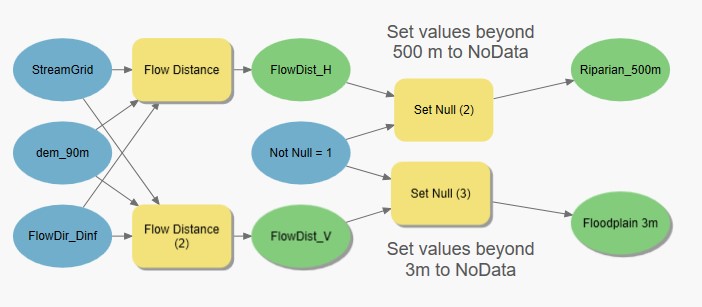
Your horizontal values should span from
0-8695.4and vertical values should span from-58-1683.28. How you get negative horizontal values, I don’t know. Perhaps filled sinks??
Summary
In these analyses, we adapted ESRI’s hydrologic tools to generate new and useful products. These will come in handy when we perform our site evaluation in the next and last section of this assignment where we assemble these layers into a site analysis of the Sierra de Oaxaca region.