Project 2 - Sierra Costera Site Evaluation (Part 2)

Overview - Part 2
In this lab, we continue our examination of terrain and ecohydrology in the Sierra Costera de Oaxaca. In the previous section, we generated hydrologic-based products. Here, we explore methods for deriving various terrain-based datasets used to depict ecological communities within our study area.
Learning Objectives
| Section | Objectives |
|---|---|
| 4.2 Calculating upstream areas | • Delineate areas upstream of a provided set of points • Understand the need to snap pour points • Describe the process of the Snap Pour Point tool and its shortcomings • Use the Snap tool to improve the Snap Pour Point procedure |
| 5.1 Topographic Convergence Index | • Describe the principles behind TCI • Convert flow accumulation to total drainage area ($a$) • Convert slope from degrees to radians & compute the tangent of slope ($b$) • Compute TCI: $ln(a/tan(b))$ • Appropriately symbolize the TCI output • Compute flow direction & accumulation using the D∞ algorithm• Compare TCI outputs derived from D8 and D∞ flow direction inputs |
| 5.2 Topographic Position Index | • Describe the principles behind TPI • Describe the workflow used to generate TPI • Understand the technique used to round floats to integers in ArcGIS Pro • Apply the TPI tool provided to generate TPI at both coarse and fine scales • Explain what inputs change to compute coarse vs fine TPI • Describe the thought process that goes into selecting a neighborhood value • Appropriately symbolize the TPI outputs |
| 5.3. Slope Position | • Explain the rational behind creating slope position products • Describe how breaks are determined for classifying TPI into slope position units • Apply the script-based tool to generate slope position from TPI • Contrast what the coarse vs fine slope position products indicate |
| 5.4 Landforms | • Articulate how landform combines coarse and fine scale TPI into a single map • Describe the various land form categories and what they indicate about the landscape • Apply the script-based tool to generate landforms from TPI inputs |
Recordings
- Proj 2.2 - Watershed delineation (23:52)
- Proj 2.2 - TCI (22:31)
- Proj 2.2 - TPI, Slope Position, & Landform (32:13)
4. Hydrologic analysis (continued from last session…)
4.2 Calculating upstream areas
In this section, we’ll continue our hydrologic analysis by looking at the technique used to delineate watersheds upstream of a given point. We’ll do this for the four gauge locations provided.
-
Add a new model in the
SierraCosteratoolbox calledUpstream tools. -
Determine catchment boundaries for a set of pour points using the Watershed tool.
- Input flow direction =
FlowD8 - Input pour point data =
GaugeLocations - Pour point field =
Id - Output =
Watersheds(in your project geodatabase)
Why do some gage sites appear to have no drainage area?
Turns out there are two potential issues going on here.
First is the extent of the analysis: by default, the watershed tool’s analysis extent is the intersection of inputs, which is likely the pour point shapefile. If your output looks like it’s constrained to a box surrounding the pour points, then set the processing extent environment to “union of inputs”.
The second issue may be that your pour points don't fall exactly on the stream. You may need to snap the pour point to an area of high flow accumulation using the snap pour point tool, or the method described below.
- Input flow direction =
-
Snap the gage sites to likely stream courses using the Snap Pour Point tool.
- Input pour point data =
GaugeLocations - Pour point field =
Id - Input accumulation raster =
FlowAcc - Output =
SnappedGages(in Scratchfoldergeodatabase) - Snap distance =
250
Inspect a few gage sites and their snapped counterparts. Evaluate how the chosen snap distance performed: should it be increased? Decreased?
- Input pour point data =
-
Re-calculate watershed boundaries using the snapped gage locations…
- Input flow direction =
FlowDir - Input pour point data =
SnappedGages - Pour point field =
Value - Output =
Watersheds(overwrite existing copy inData folderthe project geodatabase)
Do all the points have reasonably sized drainage areas now? Zoom in to Gage #3. Anything peculiar? No need to fix this for this lab, but how might you fix this?
- Input flow direction =
►An alternative method for snapping pour points…
The Snap Pour Point tools may not work effectively if you have many pour points of varying distances to streams. If you set the snap distance too low, the pour point may not reach the stream. If you set it to high you may snap to a larger stream branch than intended. The procedure I outline below overcomes some of these errors by snapping the point to the nearest stream feature – not just the cell with the highest flow accumulation. You may find this technique more useful in some situations.
-
Add the Copy Features tool to your model.
- Input Features:
GaugeLocations - Output Feature Class:
SnappedPoints.shp(in Scratchfoldergeodatabase)
- Input Features:
-
Snap the gauge locations to the vector stream features (created previously) using the Snap tool.
This procedure works best when the vector stream network was created with the “simplify polylines” option turned off.
-
Input Features:
SnappedPoints.shp -
Snap Environment: Features =
Streams.shpType =EdgeDistance =1500 meters
-
- Run the tool and view the
SnappedPointsresult. - Create a watershed raster using these snapped points. Don’t forget to set the processing extent environment to the union of inputs…
Our hydrologic geoprocessing model now allows us to create some useful datasets, all derived from a single elevation raster. Our streams raster can be used to locate riparian areas, if that’s an interest for conservation. And our watersheds dataset could serve as a useful landscape unit for various analyses.
ArcHydro is a 3rd party extension to ArcGIS that allows you do many of these DEM based hydrologic operations and more. You may see that the NSOE machines may have ArcHydro installed on them as you can see the Arc Hydro Tools in the ArcGIS toolbox: https://www.esri.com/library/fliers/pdfs/archydro.pdf
Part II
5. Terrain Analyses
Terrain analyses that go beyond slope, aspect, and hillshaded relief offer additional ecologically relevant information. These analyses point out areas in a landscape where moisture may collect, or where inhabiting plants and animals may be more sheltered from sun, wind, and rain. In this section we will examine and use existing geoprocessing models to compute three useful terrain indices:
-
Topographic convergence index (TCI) (also known as Topographic Wetness Index or TWI) calculates the upslope contributing area in relation to slope to identify relatively wet and dry locations across a landscape.
-
Topographic Position Index (TPI) examines a cell’s elevation relative to its neighbors to identify peaks and valleys within a landscape. It is scale dependent and often is calculated at multiple scales.
-
Slope position uses topographic position index to classify a landscape distinct, ecologically relevant classes based on relative levels of exposure.
-
Landforms are determined by linking features found at fine scale topographic analysis with those found at more coarse scales. Landforms are another way to classify a landscape into ecologically relevant units.
Each of these analyses is based solely on DEM data. The geoprocessing models used to calculate these are located in the ENV761\_TerrainModels.tbx file, located in your workspace. Many of these tools are based on work done by TNC’s Andy Weiss, documented here.
5.1 Topographic Convergence Index (TCI)
Topographic convergence index (TCI) is often used as a proxy for moisture as it reflects the likelihood that water will drain to and remain at a certain location. TCI is calculated as the log of the ratio of drainage area for a given pixel to the tangent of its slope:
\[ln(a / tan (b))\]…where $a$ is drainage area and $tan(b)$ is the tangent of the slope angle. We have slope, computed in degrees, and flow accumulation from which we can derive drainage area, so we can compute TCI from these. First we’ll compute TCI from our D8 flow accumulation:
♦ Topographic Convergence from D8 Flow Accumulation
-
Create a new model in your toolbox to hold TCI and other terrain analysis calculations.
-
Add the Flow Accumulation and Slope (degrees) raster datasets created earlier.
-
To compute drainage area from flow accumulation, we need to:
- Add a ‘1’ to all values, to include the cell itself.
- Then multiply all values by area of a given cell, 8100 in our case, to get a value in m$^2$. (Note, you can also compute the cell size in your model using the
Get Raster Propertiestool.)
→ Add a raster calculator tool to run these calculations. You should get values from
8100 to 1,548,242,100. (NOTE - this is slightly different than what’s in the recording - an update from 2021!) -
To convert our slope to tan(slope), we need to:
-
Convert our slope from degrees to radians (multiply by pi/180).
-
Compute the tangent of our slope, now in radians.
Add a raster calculator tool to compute
Tan(<slope in degrees> * math.pi / 180).→ The range of values in the slope raster, in radians, should be
0(or some extremely small value) to1.6684.→ The range in values of the tangent of slope (in radians) should be
0(or some extremely small value) to2.33935. Alternatively, we could just compute slope in percent and multiply by 100 which equals tan(slope)!
 -
-
Compute TCI by taking the natural log (ln) of the product of dividing drainage area by tan(slope).
Save as
TCI_D8in your project geodatabase.Values should range from
8.484to33.776. If you get different values, you perhaps set your Flow Accumulation output to be Float, not Integer in Part 1 of this lab exercise? (NOTE - this is slightly different than what’s on the recording - an update from 2021!) -
Examine your results.
Add an appropriate color ramp and set them to be partially transparent, and then display them with the hillshade map underneath. Be sure you understand what high and low values represent.
♦ Topographic Convergence from DINF Flow Accumulation
We can improve our drainage area from the one created above. That one was created using the 8-direction (D8) flow direction raster, which is still useful for deriving stream layers. However, computing flow accumulation from an infinite direction flow direction raster (DINF) will be far more precise and thus give us a better product. So…
-
Add a new model or add the following to an existing model in your toolbox for DINF TCI.
-
Compute a new flow accumulation raster derived from an infinite-direction flow direction raster (continue using Integer as the output type, for purposes of consistency).
→ Make sure you start with your filled 90m DEM.
-
Convert your d-inf flow accumulation values from cells to drainage area, in m$^2$. As above…
The values for drainage areas should range from
8100to1,548,047,700 -
Compute $ln(a/tan(b))$ using the drainage area derived from the DINF flow direction.
Save this as
TPI_Dinfin your data folder.The range of values should be:
8.334 to 33.777 -
Examine your results. Symbolize as above.
5.2 Topographic Position Index (TPI)
The topographic position index (TPI) reveals peaks and valleys within a landscape by comparing each cell’s elevation with the mean elevation of neighboring cells. A peak will be higher relative to its neighbors, and valley will be lower. Thus we simply need to subtract a pixel's actual elevation from the mean elevation of its neighbors.
Topographic position is scale dependent; the size of the neighborhood (usually an annulus) chosen will reveal different features. Smaller radii reveal a dendritic network of both main and lateral ridges as well as drainage networks. Larger radii reveal major ridge lines and drainage areas; smaller lateral features disappear.
We will compute both a fine and a coarse TPI, done by adjusting the number of neighboring cells used to generate mean elevation.
I have provided you with a tool that computes TPI, found in the supplied ENV761_TerrainModels.tbx toolbox as
Compute TPI. Before using the tool, open it up in Edit mode and examine how this tool works. Ask questions if you don't understand any of the logic or processes.To use this tool, simply drag and drop it into your existing terrain tools model, as you would any other ArcGIS Pro tool.
-
Add the
Compute TPItool to your existing Terrain Analysis model.- Input DEM =
DEM_90m - Neighborhood = Annulus with an inner radius of
1cell and an outer radius of5cells - Output =
TPI_fine(data folder)
- Input DEM =
-
Add another instance of the Topographic Position Index tool to your Terrain Analysis model.
- Input DEM =
DEM_90m - Neighborhood = Annulus with an inner radius of
20cells and an outer radius of25cells - Output =
TPI_coarse(data folder)
- Input DEM =
Run the tools and add the outputs to your display. Like TCI, set the maps to be 40% transparent and display with the hillshade underneath. View the results and play with the inner and outer radii so that the two datasets display different phenomena.
5.3 Slope Position
As described in Weiss poster on landform analysis, we can reclassify the continuous value in the topographic position result into discreet slope position classes representing functional divisions in the landscape. What values to choose to define the ranges within the reclassification depends on the topography of your area: regions with little topographic relief should use narrower ranges while areas of high relief (like ours) can use larger ones.
Weiss proposes, as a standard, repeatable method, using standard deviation units.
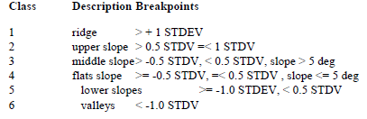
Manual calculation of Slope Position from TPI*
You can use the Get Raster Properties tool to calculate the standard deviation of a TPI raster, and then use that value to manually define the breaks in a Reclassify tool (or a series of Con statements in a Raster Calculation) to create a Slope Position dataset.
* Such a long raster calculation statement is more than likely to involve at least one typo which would be truly annoying to identify and fix. Thus, I’ve provided a Python script based tool that does the same process…
Using the provided Slope Position script tool
Because the above is not terribly sophisticated but does require a lot of typing (and room for mistakes), I’ve created a simple Python script-based tool that calculates slope position from TPI. The Slope Position (Raster Calc) tool provided simplifies this somewhat, but the script-based tool I provide is more robust. (Raster Calculator tools are notoriously finicky). We’ll use this Python-based one…
-
Add two instances the Slope Position tool (the one in the Scripts folder in your toolbox) to your Terrain Analysis model. (The tool is found in the Scripts folder of the
ENV761_TerrainModelstoolbox.) One instance will be for the fine TPI dataset and the other for the coarse TPI one. -
Link the Slope position tool with the Slope dataset and with your respective TPI dataset.
-
Run the model. Add the results to your display. Use the
SlopePosition.lyrxfile in the LayerTemplates folder to symbolize your output. (Though you still may want to set the transparency to 40% and show it on top of the Hillshade map.)→ Alternatively, use the
Apply Symbology from Layertool in your model to apply the symbology.
5.4 Landforms
Combining the coarse and fine scale TPI (with slope further dividing some classes) reveals many unique landforms within our landscape (See the Weiss poster). As in calculating Slope Position, you could do this manually using a series of nested Con statements designed to implement the set of conditions presented in Weiss’ poster:
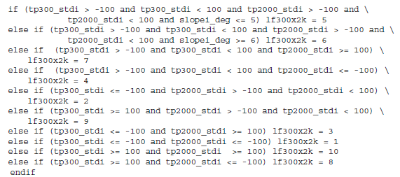
Again, however, it would be both exceedingly tedious and quite error prone to type all this out. So rather than have you do this, I have created another Python script based tool that does this quite easily.
-
Add the Calculate Landform tool to your model.
-
Set the inputs to be the slope dataset and the two TPI datasets.
-
Run the model. Add the results to your display. Use the LandForm.lyrx file in the LayerTemplates folder to symbolize your output.
♦ Summary
In doing this lab, we’ve generated a number of conservation-relevant datasets, all originating from just a digital elevation model. The techniques used here can be adjusted only slightly (with different inputs and analysis parameters) to add many more useful datasets on which we can base our prioritization decisions.
It is essential that you understand any models that you use, particularly what assumptions are made in using them and how they might affect results. Be sure to study the models in the TerrainModels toolbox noting how they work. Are any assumptions made within these models? What are the impacts of these assumptions? What could we do to validate any assumptions we make?