Lab 0 - Organizing Spatial Data
Overview
All spatial analyses require data and often generate a lot of temporary files. You’ll benefit by being organized with your data and maintaining documentation on what is what in among your files.
In this exercise, we review some best practices for managing spatial data for a project. These aren’t hard and fast rules in that you can still get valid results without following these guidelines, but based on my years of experience, I found these tips have saved me gobs of time.
We’ll explore these best practices in the context of a fabricated project. Here, I provide you with some datasets in various formats, scales, and projections. Some are well documented; others are not. Your task will be to prepare a workspace for analysis. In subsequent tutorials, we will explore where you might turn when you aren’t given the source data but rather have to find them yourself. From there we’ll review basic principles of cartography and best practices for presenting your results in map, tabular, and text format.
Learning Objectives
- Create a workspace file structure that maintains organization and is distributable
- Organize and prepare data within this workspace to facilitate analysis
- Deal with datasets that are missing projection information
- Mosaic and properly reproject DEM data tiles
- Integrate data stored in an ArcGIS Online (AGOL repository) into your project
The Scenario
Congratulations on your new job as GIS specialist for the Malagasy Conservation Group (MGC)! Your first assignment is to assist in planning the route of some newly acquired un-manned aerial vehicles (UAVs or drones) over Masoala National Park in the NE corner of Madagascar. As yet, the specific objective of the analysis is not known, but you are told to prepare the data for whatever may be asked of you.
Your predecessor has left you all the data you need, but not in a very organized fashion and with varying levels of documentation. These data sets can be found here. Your task will be to organize these files and prepare an ArcMap workspace so that you are up and running when the drone team comes to visit in the next few days.
The following steps will guide you through this process. At the end of the tutorial you will have a single project folder containing all the data you need for the analysis as well as an ArcMap document and toolbox with the proper environment settings applied. This project folder can be backed up or moved to different locations while still retaining all the data and formatting required to allow you to jump right back into the analysis.
Step 1: Create your project workspace
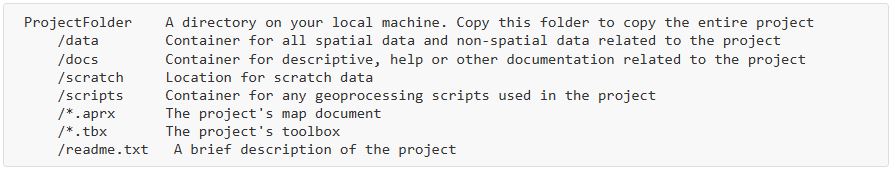
The first step in any geospatial project you begin should be to create a workspace that will keep your files organized. Geospatial analysis is notorious for making many, many intermediate datasets, themselves made up of multiple files, which can easily clutter up your machine. ArcGIS Pro has some mechanisms for handling this, but we recommend a few additional steps prior to creating your ArcGIS Pro project that will help in keeping your workspace organized. These steps involve creating a folder structure consisting of a project or root folder in which everything else is stored, and within this folder are four subfolders - data, docs, scratch, and scripts - each with a specific purpose. Once that is complete, we’ll create a new ArcGIS Pro project in the root folder and our workspace components will be complete. In the end, it will have the following structure:
-
Project folder and sub-folders Using Windows Explorer, create a project folder (we’ll call it
Lab0_Masoalafor now) and the four subfolders for your Masoala project. Always be sure that no spaces occur in the project folder name or anywhere in the path to this folder. Spaces in file, folder, and path names can cause errors when certain ArcGIS tools are run. Use underscores if you need (e.g. “My_project”, not “My project”), but avoid spaces and other odd characters. -
The readme.txt file Create a new text named
README.txtin your project folder file. Use this file to store a few comments about the workspace - enough to briefly explain what the project is about, to differentiate it from other workspaces in case you or someone else revisits this workspace from a long hiatus. Include your name and the date. -
The ArcGIS Pro project and it's components Open ArcGIS Pro and create a new blank project. Let’s name it
Masoalaand save it in a new folder on your class drive. Be sure the option to create a new folder for the project is NOT checked.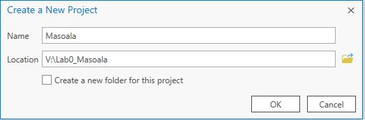
When you do this, ArcGIS Pro creates a new project file (Masoala.aprx, a default toolbox (Masoala.tbx), and a default geodatabase (Masoala.gdb).
An alternative approach is to not create the folder ahead of time and check the box here to create a new folder. Either way seems to work just fine.
-
Create a scratch geodatabase In the
Scratchfolder, create a scratch geodatabase calledscratch.gdb. You’ll have to do this from within ArcGIS Pro’scatalogpane by right-clicking on theDatabasesoption and selectingNew File Geodatabase.- This scratch geodatabase is useful when you want an intermediate dataset to be stored within a geodatabase, e.g., when you want feature area and/or length to be automatically created.
-
Set geoprocessing environment variables Finally, you’ll want to set your geoprocessing environment variables - at least the workspace variables - for your project. This is done in the
Analysismenu, from theEnvironmentstab.- Set your Current Workspace to the
Datafolder or the default geodatabase created when you created your project. - Set your Scratch Workspace to your the
Scratchfolder or the scratch geodatabase just created.
Depending on other needs of your analysis, you might want to set other environment variables, but this will do for now.
- Set your Current Workspace to the
In the end your workspace should look like this. (You may have to refresh your Lab0_Masoala folder in ArcGIS…)
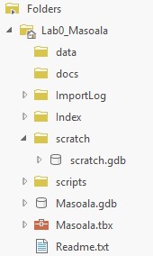
You now should have your workspace all set and should be ready to begin your analysis. Getting in the habit of starting each project by creating a workspace in this format will likely save you a lot of time and headache in the long run. You can view an example of how your workspace should look by expanding the ExampleWorkspace_Masoala.zip file.
Step 2. Organizing and preparing data in your workspace
With our workspace set, we can organize the data we need to do our analysis. All input data sets should be stored in your Data folder, but you can add subfolders if you wish to further organize your data, e.g. by source, date, type, or whatever.
Often, you will need to preprocess your data sets before you actually do any analysis with them. This can involve uncompressing files, converting formats, defining projections, reprojecting data, etc. While you will definitely want to keep the processed files, it's up to you whether you want to retain the original files in your workspace after pre-processing them for analysis. Usually, if the data sets can be easily obtained again, if necessary, and/or if they consume valuable disk space, I will delete them and just keep the data in the format I need for processing.
Study Area
The MCG has provided two geospatial data files delimiting the study extent. These are found in the MCGdata folder (in this zip file: MCG.zip). Your first task is to prepare these files and add them to your map. Also in this folder is a README_MCG.txt, which contains information about these files.
- Copy/unzip entire MCG data folder to your workspace data folder.
- Create a new map in your project
- Add the
ParkBoundary.shpshapefile to your map, then zoom to the layer. Does the feature appear to be in Madagascar, as you’d expect?? Nope. Looks like it has a projection issue.- Does this dataset have a defined coordinate system? (
Properties>Source>Spatial Reference)
- Does this dataset have a defined coordinate system? (
- Add the
LabordeGrid.shpfile. Better luck with this one?
You’ve just discovered that these two feature classes do not have any defined projections. The metadata file indicates these coverages use the “Laborde” projection, but since the coverages themselves have no defined coordinate system, ArcMap has no way of knowing this. So, the next step is to define the projection for these files.
-
Open the Define Projection tool and add the Park Boundary coverage as the input.
-
Now we need to locate the correct coordinate system to assign to these data sets.
-
Open up the Spatial Reference Properties box from the Define Projection tool.
-
The
Readme\_MCG.txtfile indicates these data use the “Laborde” coordinate system. Try searching forLabordein the Spatial Reference Properties box. -
Two Laborde projections are found. To find out which one to use, examine their properties (click on the
Detailslink in the Coordinate system window), and cross-reference the values to the ones in theReadme\_MCG.txtfile. -
Run the tool. Using a basemap, check that the results look correct; it should appear on the small peninsula in the northeastern corner of Madagascar. If not, you need to check to see that your defined coordinate system is correct. If it does, then you are finished with these data and move onto the next dataset.
-
- At this point you may wish to symbolize your data to appear more aesthetic, and to rename the entry in the map’s table of contents.
- Oh, and this is a good time to save your project!
ASTER Elevation Data
In addition to the park boundary and the quadrat grid, the drone team will also need an elevation and a land cover dataset. ASTER elevation data were given to us in their raw downloaded form as 4 zip files, each comprising 1 x 1° tiles of 30 arc-second DEMs. In this section, we will uncompress the files, mosaic the tiles into a single dataset, and reproject the data to match the Laborde projection used above.
-
Copy the
ASTERfolder from the folder to your data folder. -
Unzip one of the zip files. You’ll see it contains a README PDF file and a pair of raster GeoTIFF files. Browse the
README.pdffile to discover what the_dem.tifand the_num.tiffiles represent. -
Add the two unzipped geoTIFF files to your map; examine them and their properties.
-
Are the files georeferenced? To what coordinate system?
-
What cell sizes do they have?
-
What pixel types and depth are they?
-
Do either have attribute tables?
-
Is there any information on how they should be displayed? (e.g. a legend)
-
-
Unzip the remaining zip file. (You can overwrite the Readme.pdf files as each is identical.) As a preprocessing step, we will merge both sets of geoTIFF into single raster datasets as they’ll be easier to manage in the project.
-
Open the Mosaic to New Raster tool. Add the 2
_dem.tiftiles as inputs to the tool, and save the output to the scratch folder. Set the pixel depth to the same as the input images. Save the output asASTER_DEM.imgand run the tool. -
Repeat the procedure for the
_num.tiffiles, saving the output toASTER_NUM.img.
-
-
The remaining step is to reproject these datasets to the Laborde projection. Use the Project Raster tool to do this, saving the outputs to the data folder.
Some important aspects to note when using this tool:
- First, you will need to specify a transformation. Use
Tananarive_1925_To_WGS_1984_2. (This may appear by default.)
- First, you will need to specify a transformation. Use
-
Second, the resampling technique should not be overlooked. For categorical data (e.g. the
ASTER_NUMdataset) you should use NEAREST or MAJORITY, while for continuous data (e.g. theASTER_DEMdataset) you should use BILINEAR. Be sure you understand why.- The output cell size defaults to something near 30 m. Let’s round it to 30 m to be tidy.
When the datasets are reprojected, take a look at the output. You’ll see that you have elevation data that extends far beyond the study area.* A quick trick to subset is to set the processing extent environment variable on the geoprocessing tool. (If you don’t know how to do this, ask the instructor or one of the TAs...)
It’s your call whether you want perform the Mosaic to New Raster tool on its own or add it to a geoprocessing model in your workspace. I find it useful to add complex preprocessing steps to a toolbox, which both documents the process and provided an easy way to repeat the steps if necessary.
We now have ASTER DEM data (and their corresponding quality control rasters) for the extent and in the coordinate system of our analysis. To conserve space, we’ll delete the original GeoTIFF files and their compressed counterparts. In the end you should only have 8 files in your folder.
Land cover data
- With the Catalog frame active, select the Portal tab, then select the cloud icon with no objects. This allows you to search the public contents of ArcGIS Online for data.
- Search for:
Africa Land Cover owner:consbioFrom the results, view the details for the “Land cover, Africa and the Arabian Peninsula”. Review the details and then right-click and add this dataset to your map. (It may take a few seconds…) - When added to your map, view the layer’s properties to determine where the data are stored on your local machine. Note that it’s on the
C:/drive, and thus won't be available to you if you move machines. - Make a local copy of the relevant land cover data, i.e., just the data for the extent of your study area. You can use the extent of either of the ASTER datasets to define this extent.
- Project the dataset to the Laborde projection. While the input data has a cell size of 300m, set the output to 30m to match the DEM dataset. Also be sure to use NEAREST (or MAJORITY) as the resampling technique and [set the processing extent to the Laborde Grid shapefile.
- Set the symbology of the projected output dataset to match the LYR file from the ArcGIS Online derived dataset.
Testing your workspace
- Close your ArcGIS project and delete all files from your scratch folder.
- Copy your entire workspace to a new location or rename the root folder.
- Open your map an all the data should appear as you left it.
Recap / What’s next
At the end of the exercise you have a tidy, efficient workspace ready for analysis. All the data is organized and in a single projection, which will greatly simplify analysis and minimize errors. In later exercises we will explore how you might assemble a dataset when the data are not simply given to you.