Habitat Modeling - Part 1: Building the Model

Background

Last week we examined a few techniques for deriving several useful datasets from digital elevation model data. These derived datasets gave us clues to where we are likely to find higher biodiversity (hot and wet areas), but by themselves they don't reveal much about what particular species are likely to be found in any given location. In this exercise, we focus on the spatial analyses (and to some degree the statistical analyses) used to do just that: to map out the habitat for a given species.

Habitat mapping, also called species distribution modeling, is an indispensable tool for conservation since we usually want to focus efforts where species of concern actually exists or where biodiversity is high. The techniques learned here, however, have additional applications, as they can reveal not only where species are likely to be found, but also where other natural resources might occur or even thrive. For example, the Pennsylvania TNC used habitat modeling techniques to predict where new hydraulic fracturing wells are likely to be placed so they could model their impact on forests (source).

Approaches to habitat modeling

There are a few approaches to habitat modeling; which one is appropriate for a given situation depends on what is known about the species and the quality and abundance of data available for an analysis.

Perhaps the most historically widespread approach to habitat modeling is expert based mapping. This is where people who are very familiar with the known range of the species (i.e. experts) can draw that range on a map with a reasonable degree of confidence. These maps are common in biological atlases and can be viewed for many species through NatureServe's / InfoNatura's portal (LINK). While the quality of expert based maps is only as good as the knowledge held by the expert(s), and some may be of dubious accuracy, the maps are often the best information available and can lead to better conservation decisions than without them.

A second approach to habitat modeling is generative or rule-based mapping. This approach is also informed by expert knowledge, but instead of knowledge where the species has been observed, the knowledge is more about the requirements and limitations of the species. For example, perhaps it's known that the species lives within a certain elevation range, is seldom found too far from water, and needs trees to build its nests. With that information, we can create a set of spatial rules that meet these criteria with the result being a map of that species' habitat. As above, this approach is only as good as the knowledge that goes into it -- and the spatial data on which these rules are applied. However, the result can be an improvement over the expert drawn maps as it may pick up nuance that is overlooked by the drawn map.

The third approach, discriminative or statistical based mapping, is the most complex and the most objective. This approach is more useful when little is known about the species, but it requires at least a few known locations where species has been observed, and is most accurate when a thorough survey is conducted to provide data on both known locations and known absences of the species. These locations are used to run statistical analyses on various spatial datasets representing environmental factors thought to influence habitat preferences to tease out (1) which of those environmental factors is important and (2) what values of those factors deemed important define suitable habitat for the species in question.

The statistical approach to habitat mapping continues to evolve as more methods are developed and as computational power improves. We will not be going too deep into the various statistical approaches in this lab exercise - that is more a topic for a statistics course than a spatial analysis one. Instead we will concentrate more on the overall structure of the statistical based analysis and the role GIS plays in generating the data for these statistical models as well as interpreting and evaluating the results.

Context of our analysis:
The pygmy salamander (Desmognathus wrighti)

In this exercise we will be developing a habitat model for the pygmy salamander found in the southwest corner of North Carolina. However, our overall goal will not be so much to generate a "bullet proof" habitat map for this species as it will to (1) explore what environmental factors influence this species, and (2) understand the role GIS/spatial analysis plays in modeling this species' habitat.

The exercise consists of three parts. The first part involves getting to know the species. Any clues as to what biophysical factors might shape the salamander's habitat can help us narrow our search for supporting data and improve our results. Second, we will develop a rule-based model informed by "expert knowledge" provided to us. And third, we will use MaxEnt, a popular statistics-based habitat modeling package - to generate a habitat suitability map based on occurrence locations and environmental data.

We will be following this lab up next week with further analysis of our salamander habitat models. In that exercise we will be evaluating how well we think our models did and interpreting the result to improve our understanding of the salamander and ultimately arrive at a habitat map of the species.

Data used in this exercise

The SDM_Exercise.zip file includes both a set of known locations where the pygmy salamander has been observed as well as a set of spatial datasets that can be used as environmental layers (or to generate environmental layers) for both deductive and statistic-based habitat mapping.

SDM_Exercise.zip contents:

• A raster mask marking the extent of your analysis
• 1 arc-second DEM raster (NED)
• 2011 land cover raster (NLCD)
• GAP land cover raster (SE Regional Gap Analysis Program)
• 1 km modeled precipitation and temperature data raster (PRISM)
• Pygmy salamander element occurrence data (NC Wildlife Commission)
• Some useful geoprocessing tools to kick start your analysis
• MaxEnt software folder

While the spatial data are public domain and you are welcome to re-distribute these data freely, the salamander occurrence records are provided by permission only and should not be used outside this lab exercise.

Deliverables

While there is nothing to submit for this week's lab assignment (it will all be submitted next week, after we've done our model assessment), the following products will be good milestones for your analysis.

• A short description of the biophysical features that may be relevant in modeling your species.
• A listing of the spatial datasets that are useful proxies for these biophysical features
• A geoprocessing toolbox used to run a rule-based model for your species
• A geoprocessing toolbox used to generate the inputs formatted for MaxEnt
• Your MaxEnt results
• Habitat range maps for the species derived from the rule-based and MaxEnt models

PART I - Preparation and background

Step 1.1. Preparing your workspace

• Create a workspace using the standard format we've been using (project folder with Data, Docs, Scratch, and Scripts subfolders, etc.).
• Extract the contents of the SDM_Exercise.zip file and move contents to the appropriate directory. (MaxEnt files can go either in the root folder or the Scripts subfolder.)
• Create a new ArcGIS Pro project document. Add the toolbox provided in the zip file as well.

Step 1.2. Compile information on the species (ecological model...)

The first step in any habitat modeling exercise is to become as familiar as you can with the species you are modeling. In the framework presented by M.P. Austin (2002), this constitutes our ecological model. This model helps guide the analysis and likely make your work more efficient and productive. There are a few useful sites for finding general information, and even some distribution data, for species. These include:

• IUCN: http://www.iucnredlist.org/details/59259/0
• NatureServe Explorer: http://www.natureserve.org/explorer/servlet/NatureServe?searchSciOrCommonName=Desmognathus+wrighti+&x=10&y=12
• Amphiweb: http://herpsofnc.org/?s=Desmognathus+wrighti
• Crespi, et al (2003): http://onlinelibrary.wiley.com/doi/10.1046/j.1365-294X.2003.01797.x/pdf
• Animal Diversity Web: http://animaldiversity.ummz.umich.edu/accounts/Desmognathus_wrighti/

From these sources, you can determine the following information about the pigmy salamander...

• It's usually observed between 1600 and 2012 m in elevation, but has been seen as low as 762 m.
• It's often found near spruce fir stands at higher elevations, and mesophytic cove forests at lower elevations.
• While it's entirely terrestrial, 76% of the observations were within 61 m of streams.
• It hides under moss, leaf litter, logs, bark, and rocks.
• It hibernates in underground seepages.
• There may be two distinct populations, one northern and one southern

Step 1.3. Generate a list of [possibly] relevant environmental variables (data model...)

So, with this background, we can generate a more informed hypothesis about our species. For example, we see that elevation is important (though we can only speculate why: temperature?). Furthermore, we have some general vegetation associations to narrow in on, and we see that moisture is important as the salamander needs seepages for hibernation. We are not aware of any direct relationships with the solar exposure or slope, though those factors may have important indirect contributions to temperature. There may well be other factors, but our first-hand information is limited.

The ensuing step is to generate our data model, i.e. to see what spatial data sets we might have or could generate that could serve as proxies for the above conditions. Elevation is an obvious one. A vegetation map of the thematic resolution that identities the classes important to a salamander, if available, would be another useful data set. For the moisture constraints, we aren't likely to have a map of underground seepages, but perhaps a soils map or one of our DEM based moisture maps could prove useful. (Yes, we are simplifying things a bit here, but for the purposes of the exercise, this should be fine...)

Step 1.4. Build a geodatabase of [possibly] relevant environmental variables

It's here where we apply the skills developed in the previous class section to use. We want to assemble a geospatial database to include the best proxies for the environmental conditions outlined above. Knowing that you could do this on your own, I've opted to save time and provide the raw data for you. These include a 1 arc-second DEM from the National Atlas, land cover from two sources - the 2011 NLCD and the Southeast Regional GAP program, and climate data (monthly temperature and precipitation) from Oregon State's PRISM data set. Additionally, I've digested a few of these datasets to move the analysis along.

What's been done for you...

The elevation and NLCD data have been downloaded from the National Map and projected to the UTM Zone 17 (NAD 83) coordinate system at a 30 m cell size. The SE Regional Gap Vegetation data was also subset for the study area and projected to the UTM Zone 17 coordinate system at a 30 m cell size). The process I used is captured in the geoprocessing model named "A. NED, NLCD, GAP preprocessing" found in the ENV761_HabitatModeling toolbox provided to you. The raw data files are not provided to you, but can be made available.

The PRISM climate data, which include mean monthly precipitation, minimum monthly temperature, and maximum monthly temperature (a total of 36 data layers) were summarized into bioclimatically relevant layers. These include mean monthly precipitation, precipitation of the driest month and of the wettest month, as well as mean minimum monthly temperature and mean maximum monthly temperature (a total of 5 summaries). These climate summary data sets, calculated in their native coordinate system (WGS 1972) and cell size (1 km), were projected to the UTM Zone 17 coordinate system while downscaling the cells to 30 m using a bilinear interpolation. The cells were downscaled to match the cell size of the other raster layers. The process I used is captured in the geoprocessing model named "B. PRISM Summaries" found in the ENV761_HabitatModeling toolbox provided to you. (Again the raw data files are not provided, but can be made available.)

NOTE: The units of these PRISM datasets are in mm x100 and °C x100 for precipitation and temperature, respectively. (So a cell value of 2300 in the PPTMax dataset is 23 mm of precipitation).

What you need to do...

Later in our analyses, we'll be exporting all our environment rasters into a MaxEnt compatible format (ASCII). As you'll see later in this exercise, putting all our rasters into a single geodatabase will facilitate this step, so:

• Create a new file geodatabase in your project workspace called EnvVars.
• Copy your NED30 and SEReGAP rasters (which have already been clipped to the proper extent) into that geodatabase.

While a good deal of the data assembly was done for you, you still need to subset the NLCD and PRISM datasets (so that all share the exact same extent, as well as to conserve disk space) and derive any additional datasets you require. If you begin by subsetting the data, then any derived datasets should match the extent as well. So begin there.

• Subset the NLCD and PRISM data sets to the extent of your AnalysisMask.img dataset. Make sure the outputs go to your EnvVars geodatabase.

From here, we'll compute a number of other derived datsets

• Create DEM-derived datasets

  • Slope (percent rise)
  • Northness: Cos([Aspect] * math.pi/180)
  • Eastness: Sin([Aspect] * math.pi/180)
  • Insolation
  • TPI_250 (annulus with 30/250m inner/outer radii)
  • TPI_2000 (annulus with 1500/2000m inner/outer radii)

• Create a stream raster, as we did in previous labs, assigning streams as flow accumulation > 1000 cells.

• Distance to Stream: Euclidean distance from these streams.

♦ Conduct a neighborhood analysis on forest cover types

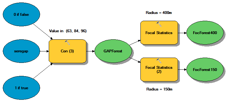
Another dataset we will create is neighborhood percentage of important forest layers. This is created by first extracting the classes from the GAP land cover dataset likely to be good salamander habitat (classes 63, 84, and 96) into a binary raster ('1' if it is one of those classes; '0' if not), and then calculating a neighborhood mean on that raster. The result will be the percentage of cells within the neighborhood radius that are within the specified classes.

This data set is potentially useful for two reasons. First, since class boundaries are seldom exact in any land cover map, this "smooths" the data a bit, allowing habitat to include pixels that are not just classified as the selected forest type, but also those that are in close proximity to them. Second, if we use this environmental layer in any inductive, or statistics-based, model (which we will), this alleviates the issue that an observation location may be imprecise, in which case the land cover class extracted for a given sample would be completely off (for example a meadow one cell away from proper forest cover).

When creating a focal forest layer, there is the question of what to use for a focal radius. As we don't have much information to go on, we'll try two distances.

• Create focal forest layers for SE Regional GAP cover types 63, 84, and 96 - one using a radius of 150 m and one with a radius of 400 m.

You should now have 17 raster datasets representing your environmental layers all in a single folder. That folder should look like this in ArcCatalog (though your names may be different):

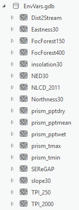
Furthermore, each of these rasters should have the same extent and cell size as the Analysis mask. If you open up the properties of each and click on the Source tab, they should show they have 3187 columns and 3051 rows in the Raster Information setting.

Once these rasters are created, we are ready to begin map the salamander's habitat using an arsenal of rule based and/or statistical approaches.

PART II - Rule-based modeling

Rule-based habitat models, also referred to as generative or envelope models, are the oldest and simplest habitat models. They consist of defining the limits of different environmental conditions in which one would expect to find a species - the so-called "Hutchinsonian hypervolume". The trickiest part of these rule based models is defining the limits. This is most often done using expert knowledge about the species, but could also be done using observation data to chart - in parameter space - the ranges in which the species has been observed. Envelopes or Mahalanobis distance metrics can be applied to these values to confine the hypervolume, but once the boundaries are specified, the spatial component is relatively easy.

In our exercise, we will rely on "expert knowledge" about the pigmy salamander. We'll use this knowledge to set the rules and then use some raster algebra to apply those rules to come up with habitat map for our species.

Step 2.1. Setting the rules

From our background research as well as meetings with pigmy salamander experts, we've deduced the following constraints on our salamander.

• Salamanders are found above 762 m in elevation and below 2012 m.

• Salamanders prefer areas that are within 400 m of the following GAP cover classes:

  • Class #63 - Central and Southern Appalachian Northern Hardwood Forest
  • Class #84 - Southern and Central Appalachian Oak Forest
  • Class #96 - Central and Southern Appalachian Spruce-Fir Forest

• Salamanders require places where the max monthly temperature never exceeds 18° C.

• Salamanders occur in places where the driest month gets at least 96mm of precipitation.

Step 2.2. Applying the rules

Given this information, we can fairly easily extract the pixels that meet these criteria using raster calculations in a geoprocessing model:

1. Create a new geoprocessing model. Name it "Rule Based Model"
2. Add the elevation, focal forest (400m), PRISM max monthly temperature, and PRISM driest month precipitation layers to the model.
3. Add the Raster Calculator tool and assemble the following calculation. You may want to do this piecemeal, running the tool after each chunk to make sure you have no typos. You should end up with a raster output containing 1's (where all the criteria are true) and 0's where any of the criteria are false. If you end up with only zeros, check your statement.

([Elevation]> 760) & ([Elevation] < 2012) & ([FocalForest400] > 0.5) & ([Tmax] < 1800) & ([PPTdry] > 9600)

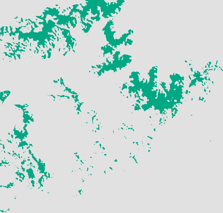
The output is your rule-based prediction. It is the spatial representation of the conditions that the experts believed to be real constraints on the salamander's habitat. Your result should resemble this:

PART III. - Statistical Modeling using MaxEnt

To complement our rule-based habitat model, we'll use a statistical approach as well. There are a wide variety of statistical approaches available, GLM, GAM, and CART to name a few. In the interest of time (and also given that this is a GIS course, not a course on statistics), we are going to focus on one of the more popular and robust statistical analysis approaches: MaxEnt.

MaxEnt, released in 2004, uses a maximum entropy approach to determine whether a location is likely to be habitat and what is not. Since its release, MaxEnt has become one of the more popular and widely used species distribution modeling software -- and for good reason. MaxEnt is robust and easy to use, it provides insightful output, and it often outperforms other modeling approaches, particularly when observation data is scarce (Elith et. al., 2006).

MaxEnt uses a complex suite of statistical analyses, combining the strengths of neural networks, GAMs, GLMs, envelope models, machine learning -- pretty much the kitchen sink of species distribution modeling -- into a single "black box". It's beyond the scope of this exercise to delve into the mechanics of this black box. For that, I encourage you to familiarize yourself with the MaxEnt "brief" tutorial (40 pages is not exactly brief...) and Elith, et. al. (2011); these are the two most explanatory sources on the MaxEnt approach. Dean Urban's notes on MaxEnt are also posted on Sakai.

In this exercise, we'll have a chance to explore some of the nuances of the MaxEnt approach, but mostly we'll be looking at how ArcGIS and MaxEnt work together to provide a useful means for generating species distribution maps -- and understanding more about the ecology of our species.

Step 3.1. Downloading the MaxEnt software

Prior to running this exercise you need to download the MaxEnt executables. The MaxEnt folder contained in the Exercise3_data.zip contains these. Alternatively, you can download them for free from the MaxEnt web site. The contents of the MaxEnt folder are as follows:

• Maxent.jar The MaxEnt executable file. (MaxEnt is written in Java.)
• Maxent.bat A batch file use to run MaxEnt with specific memory settings
• readme.txt A readme file with details on the version of MaxEnt used here
• LinkToMaxent A link to open the MaxEnt home page in a web browser

Step 3.2. Data preparation

As it is an inductive model, MaxEnt requires two sets of data: species occurrence points and the environmental layers used to discriminate habitat from non-habitat. MaxEnt is touted to be a "presence-only" platform, and as such we do not need to provide any absence (or even pseudo-absence) data -- another advantage of the MaxEnt approach. Here, we discuss the format that MaxEnt requires these inputs to take and how to generate them from the data we already have in our ArcGIS workspace.

Creating the species location file

The first step in running MaxEnt is to generate a list of presence localities, or "samples". In its simplest form, this is simply a CSV file with three columns: a species column listing the name of the species that a given sample represents, and columns for the X and Y coordinates. The order of the columns is important: the species column must always come first, followed by the X coordinate and then the Y coordinate. An example is shown below (this example is from the sample data that comes with MaxEnt).

species,longitude,latitude

bradypus_variegatus,-65.4,-10.3833

bradypus_variegatus,-65.3833,-10.3833

bradypus_variegatus,-65.1333,-16.8

bradypus_variegatus,-63.6667,-17.45

bradypus_variegatus,-63.85,-17.4

You can have as many species as you want in your samples file, as long as they are labeled uniquely in the first column. MaxEnt will allow you to select individual species (or all species) when you run an analysis. So, our first task is to create this CSV file for our salamander.

You can generate this easily from the PigmySalamander\_South.shp shapefile by exporting its feature attribute table to a CSV text file using the Copy Rows tool, being sure to give the filename a .csv extension. You can then edit the resulting text file in Excel to (1) add a column for species name and (2) delete/re-order the columns so that the X ("easting") and Y ("northing") fields follow the species name.

Note: if your attribute table did not contain the X and Y coordinates, use the Add XY Coordinate tool...

Creating the ASCII format environmental layers

Our next objective is to convert all the environmental rasters that we created in the first lab into a format that MaxEnt can read, which is ASCII format. The one major catch in creating these ASCII rasters is that for them to be read into MaxEnt, they must have the exact same cell size, alignment, and extent. Furthermore, since MaxEnt will use these ASCII files to extract values at our sample locations, these rasters must have the same coordinate system/projection that our sample coordinates use. Fortunately, as we took extra care in setting the proper environment variables when we created our environmental layers, this should be a relatively straightforward task.

You could create a new geoprocessing model and add 16 instances of the Raster to ASCII format, but there's an easier way with a simple advanced modeling trick. To do this:

1. Create a new geoprocessing model and add one instance of the Raster to ASCII tool.
2. Then from the Insert panel of the Model Builder toolbar, add the Iterate Raster iterator to your model. This will add a means by which you can iterate through all rasters in a given workspace.
3. Open the iterate Rasters object in the model and specify your EnvVars.gdb geodatabase containing all your environmental variables. Leave the remaining options blank. The output to this object now appears to be the first raster in your folder. Connect this to your Raster to ASCII tool.
4. Open up the Raster to ASCII tool and set the output to go to a new, empty folder. (e.g. create a new folder called ASCII in your Data folder and select the output to go in there. For the file name, enter %name%.asc. The result should resemble this:

What this does is iterate through each raster found in the folder you specified, convert it to raster and, with each iteration, the "Name" variable contains the current raster the model is processing (e.g. "Aspect30" for the first run, then "dist2strm", etc.), and the output is given this name.

Run the model and you should have 16 ASCII files in your ASCII folder when complete.

Step 3.3. Running MaxEnt.

MaxEnt can be run by double-clicking the maxent.jar file in your MaxEnt folder. Another way to start MaxEnt is to double click on the maxent.bat file. Why the difference? Well, the maxen.bat file just calls the maxent.jar file, but the maxent.bat file can be edited in a text editor to run MaxEnt with more than the default 512 Mb of RAM allocated to it. The machines in the ICL and ACL have 8 GB of RAM, and we can run MaxEnt a lot faster if we allow it to consume more memory when its run. To do this we edit the maxent.bat file, changing the 512 Mb to 2048 Mb so it runs with 2 Gb of memory instead of ½ Gb.

3.3.1. Running MaxEnt with more memory

1. Edit the maxent.bat file in a text editor.
2. Change "512m" to "2048m"

1. Save and close the maxent.bat file.
2. Double-click the maxent.bat file to run MaxEnt.

MaxEnt should now appear and we're ready to set up our analysis

3.3.2. MaxEnt inputs and run-time settings

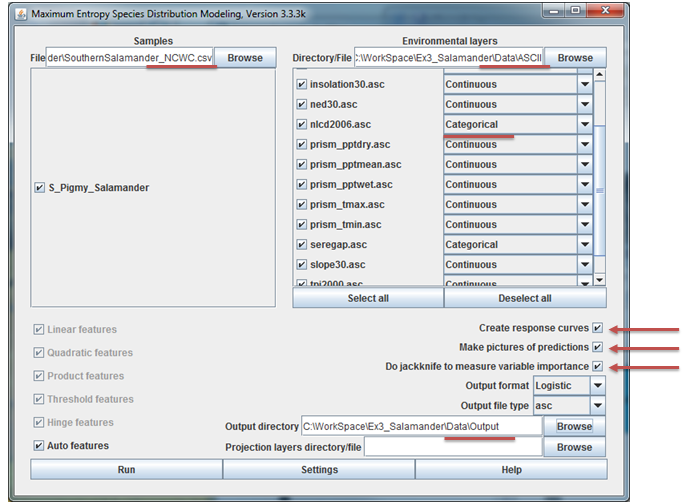
With MaxEnt up and awaiting our command, we now have to specify the samples file, the folder containing our ASCII format environment variables, and output folder, and a few run-time settings. These steps lead us through this process:

1. Specify the samples dataset by browsing to the csv file we created in the data preparation section above. You should see the salamander species appear with a check box next to it. Keep all selected as we'll run all species simultaneously.

2. Specify the folder containing all your ASCII formatted environment layers. When entered, a list of all the rasters in the folder will appear, each with a check box next to them. Notice that you can add categorical data in MaxEnt. Make sure that you set the two land cover datasets to be categorical data.

3. Specify an output folder. In specifying this folder, you can create a new folder. Create a new folder in your MaxEnt folder and set all model output to go here.

4. Set the following run-time settings:

   a. Check the box to create response curves

   b. Check the box to make pictures of predictions

   c. Check the box to do jackknife to measure variable importance

   d. Keep output format as Logistic

   e. Keep output file type as asc

The MaxEnt application should resemble the figure below. When all is set, hit Run. You may see a few errors for field names that were not used and perhaps for a few points falling outside of the environmental extent. You can just ignore these. The program should finish in about 5-10 minutes or so.

Step 3.4 Model interpretation

MaxEnt generates a lot of output, all indexed through a web page created in your output folder. Here we'll run through the highlights of the output. Your report may have slightly different values as each run of MaxEnt extracts a random sample of background points, but they shouldn't be too different. Open up your S_Pigmy_Salamander.html file in any web browser and follow along...

Pictures of the model

For now, we're going to skip the first two graphs ("Analysis of omission/commission" and "Sensitivity vs. 1 -- Specificity") and the first table. We'll come back to those when we discuss model assessment in a future exercise. Instead, scroll down to the map of the study area painted in blues to reds ("Pictures of the model")

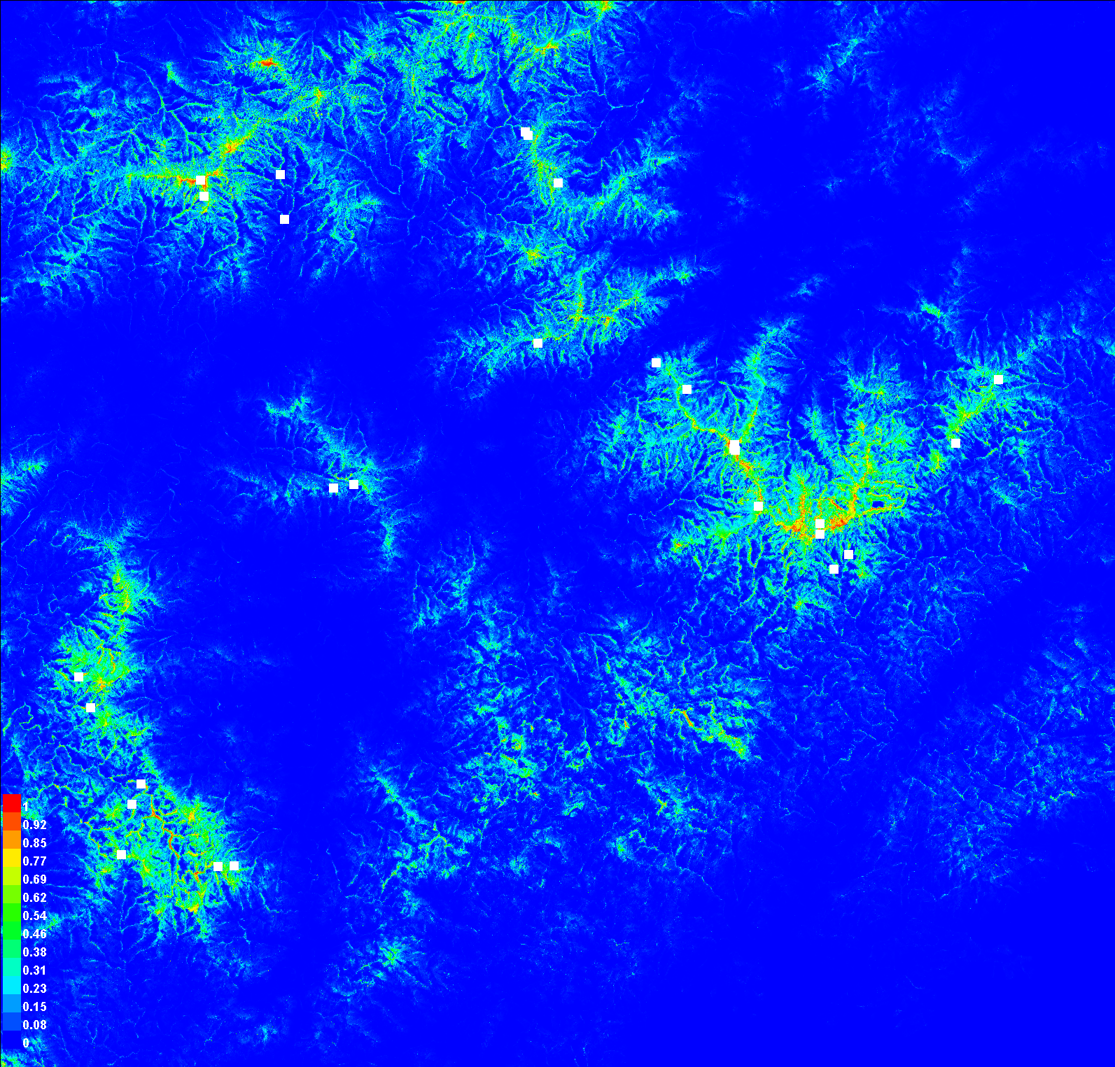
This is our habitat suitability map as predicted by MaxEnt. The values range from 0 to 1. The closer a cell's value is to 1 (the warmer colors), the more confident we are that the pixel represents suitable habitat. This is not quite a habitat map, as we still need to decide on a cutoff for what we want to be habitat or not, but we'll get there. First, let's explore how MaxEnt arrived at this map.

Response curves

Scroll down to the section on Response Curves. The first group shows the marginal response curve for each environmental variable. In these line graphs, the X axis reflects the range of values for the given environment variable and the Y axis reflects the likelihood of habitat at that given range. Flat lines indicate that the variable has no real influence in predicting what's habitat or not. The shape of the response curve reflects the various methods that MaxEnt uses to model responses (categorical, linear, quadratic, threshold, hinges, and/or interactions). As an example, have a look at the "prism_pptdry.asc" response curve (below). This appears to be a hinged response suggesting that habitat preference increases steeply as rainfall of the driest month approaches 145 mm, and then drops off considerably.

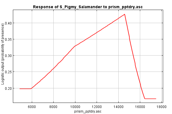
Marginal response curves are generated by keeping all the other variables at their mean. This allows some introspection of the combined interaction among variables. However, as the MaxEnt tutorial states, if two variables are correlated, like elevation and MAT often are, then a marginal difference would be difficult to see, and thus the response curves could be misleading.

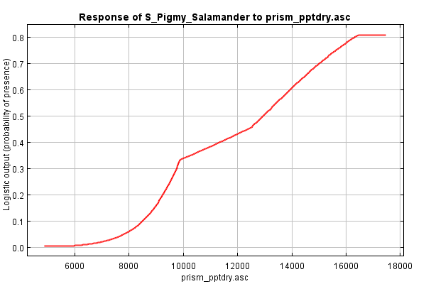
So then we examine the next set of response curves, the dependence response curves. These curves are generated using only the corresponding variable; all others are ignored. Thus, the response fails to reveal any interactions among variables, but does show a single variable's contribution to the overall prediction.

Take a look at the dependence response curve for precipitation of the driest month. This shows that, when considered in isolation of other variables, the salamander seems to prefer wetter areas. Furthermore, this preference increases rapidly up to around 100mm, and then the influence, though still strong, wanes a bit.

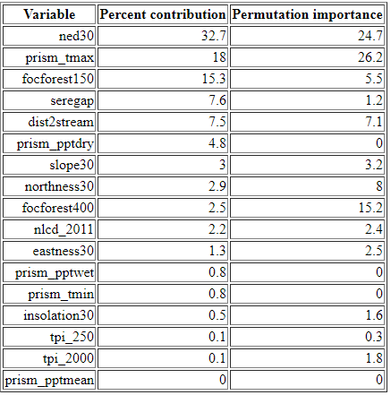
Analysis of variable contributions

In this section of the MaxEnt output file, we can see the relative importance of each environment variable in driving the final habitat suitability surface. The table lists each variable in order of its percent contribution to the model's gain. Gain is a measure of improvement to the model's ability to separate habitat from background, i.e., from retaining areas that include the values specified in the occurrence locations but removing all other areas (or "background"). As the MaxEnt tutorial cautions, the percent contribution listed in the table should not be over-interpreted as they reflect just one pathway to an optimal solution (and there may be many). Still, the table does provide at least a rough guide showing which variables appear to be important in determining habitat for a given species.

The jackknifing figure (below) provides a different view of the relative importance of the different variables. In the figure below for our salamander, the short dark blue bar for aspect30 indicates that it, by itself, contributes very little gain (or ability to separate habitat from background). Conversely, ned30 , which has the longest dark blue bar, contributes the most to gain. We can interpret this as: if we were limited to choosing only one variable to parse habitat from background, we should chose elevation of as it would give us the best single-variable model.

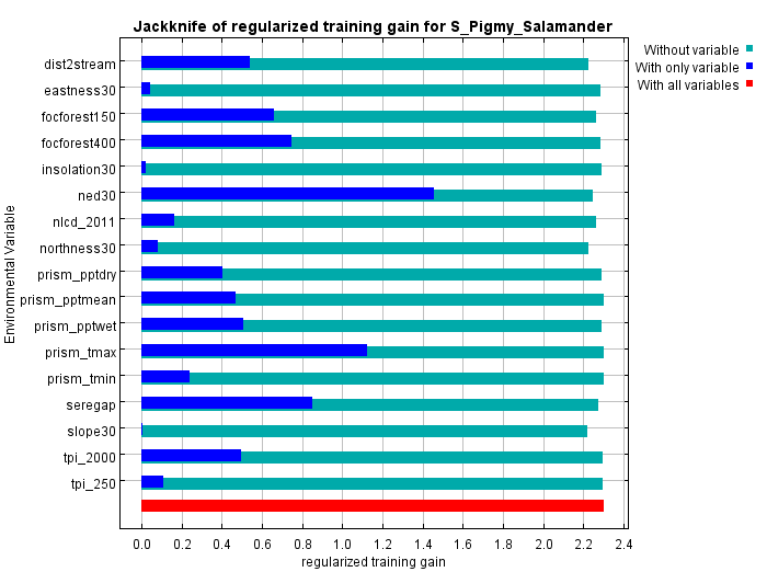
The lighter blue bars show the decline in gain if a variable were omitted. It's a way of spotting whether a variable contributes something unique to the solution. In our example, slope, or perhaps distance to stream, shows the biggest drop in gain when omitted implying that, when it's removed, there's no other environment variable that captures its contribution to gain. However, the difference is slight suggesting that the impact wouldn't be too large if the variable were omitted.

Model Interpretation: Overview

The key product from our MaxEnt analysis is the ASCII format raster of representing habitat likelihoods which we will shortly pull into ArcGIS. But the above digest of what variables are important and their response curves are also quite useful in understanding the ecology of each species distribution. Knowing the relative importance of a given environmental variable gives us insight into what factors may be constraining our species' distribution. And knowing the response curve gives us an idea how: is it a monotonic relationship? Or is there one or more "sweet spots" that the species seem to prefer.

In the case of our salamander analysis, we see that the elevation, maximum monthly temperature, and GAP land cover stand out as providing the most gain when modeled alone and leads to the largest decline in gain when omitted. So it seems that these factor seems to be important to the salamander.

Step 3.5 Mapping the results

The last remaining step is to bring MaxEnt's logistical output, in the form of an ASCII raster, back into ArcGIS, and then apply a threshold to map the habitat ranges for each of our species.

1. Create a new geoprocessing model to process the MaxEnt outputs
2. Add and instances of the ASCII to Raster tool and link it up with the.asc file in the output folder from your MaxEnt run. Be sure to set the Output data type to FLOAT.
3. The ASCII files generated do not know what coordinate system they are in, so we need to define that. Add a Define Projection tool at the end of each ASCII to Raster tool to define the outputs to have the projection used by our other datasets.

Run the model and view the MaxEnt logistical outputs. Values in these rasters should range from 0 to 1, with the higher values indicating a higher likelihood that the pixel is "habitat". The next step is to apply a cutoff. The decision where to draw the line between habitat and non-habitat is not arbitrary and depends on the sensitivity and specificity of the model (terms we'll discuss shortly). We'll discuss model tuning in a future lecture, but for now I'll just point you to the value in the MaxEnt results that gives us a good cutoff.

If you scroll to the top of your species' MaxEnt report, to the table that list Cumulative threshold, you'll see a series of logistic thresholds for different criteria. The table for our salamander is shown below.

These logistic thresholds (column 2) are the cutoffs to separate habitat from non-habitat, and the one most often used is the second from the last, the "Balance training omission, predicted area and threshold value".

The remaining steps are to use these thresholds in SetNull commands to isolate cells that are ranges for our given species. The result will be our species range maps derived from MaxEnt.

What's next

Next week in the continuation of this lab, we will review the techniques presented here and focus in on the assessment and interpretation of our distribution models. Ultimately, you will submit a brief report assessing your habitat model of the pygmy salamander.

References

Austin, M.P. (2002), Spatial prediction of species distribution: an interface between ecological theory and statistical modeling. Ecological Modelling, 157: 101-118. http://www.sciencedirect.com/science/article/pii/S0304380002002053

Elith, J., et al. (2006), Novel methods improve prediction of species' distributions from occurrence data. Ecography, 29: 129--151. (http://onlinelibrary.wiley.com/doi/10.1111/j.2006.0906-7590.04596.x/abstract)

Elith, J, et al. (2010), A statistical explanation of MaxEnt for ecologists. Diversity and Distributions, 17: 43 - 55. http://onlinelibrary.wiley.com/doi/10.1111/j.1472-4642.2010.00725.x/pdf

Phillips, S. (2006), A brief tutorial on Maxent. AT & T Research. (http://www.cs.princeton.edu/~schapire/maxent/tutorial/tutorial.doc)